link_prediction with GNN
This algorithm is available again, starting with MAGE version 1.22. The algorithm was unavailable in MAGE from version 1.14 to version 1.21.
Link prediction can be defined as a problem where one wants to predict if
there is a link between two nodes in the graph. It can be used for predicting
missing or future links in the evolving graph. Using the notation G = (V, E)
for a graph with nodes V and edges E and given two nodes v1 and v2, the
link prediction algorithm tries to predict whether those two nodes will be
connected, based on the node features and graph structure.
Lately, graph neural networks have been often used for node-classification and link-prediction problems. They are extremely useful in numerous interdisciplinary fields of work where it’s important to incorporate domain-specific knowledge to capture more fine-grained relationships among the data. Such fields usually involve working with heterogeneous and large-scale graphs. GNNs iteratively update node representations by aggregating the representations of node neighbors and their representation from the previous iteration. Such properties make graph neural networks a great tool for various problems we in Memgraph encounter. If your graph is evolving in time, check TGN model that Memgraph engineers have already developed.
In this includes the following features:
- Support for homogeneous and heterogeneous graphs.
- Support for disconnected graphs.
- Its applicability to use it as a recommendation system.
- A semi-inductive link prediction setup where a larger, updated graph is used for the inference.
- An inductive link prediction setup in which training and inference graphs are different.
- A transductive graph splitting (training and validation sets).
- Graph attention layer aggregates information using an attention mechanism from the first-hop neighbourhood as introduced by Velickovic et al..
- GraphSAGE layer extends the usability of graph neural networks to large-scale graphs as introduced by Hamilton et al..
- mlp and dot predictors are used for combining node scores to edge scores.
- ADAM and SGD optimizers are used for training neural networks.
- Support for batch training.
- Parallel graph sampling is done using multiple threads.
- Negative graph sampling is a sampling where the final graph consists only of edges that don’t exist
- Evaluating the model’s training performance using a variety of metrics like AUC, Precision, Recall, Accuracy and Confusion matrix.
- Evaluating the model’s recommendation performance with Precision@k, Recall@k, F1@k and Average Precision metrics.
When using link prediction be careful about:
- Features of all nodes should be called the same (e.g., saved as ‘features’ property of nodes).
- The model’s performance on the validation set is obtained using transductive splitting mode, while inductive dataset split is not yet supported. You can find more information about graph splitting on slides of Graph Machine Learning course offered by Stanford.
- To improve performance, self-loop is added to each node with the edge-type
set to
self. - You can set the flag to automatically add reverse edges to each existing edge and hence, convert a *directed graph to a *bidirected one. If the source and destination nodes of the edge are the same, reverse edge type will be the same as the original edge type. Otherwise, the prefix rev_ will be added to the original edge type. See the FAQ part to further see why self-loops and reverse edges are very important in ML training and how you can get into problems if your graph is already undirected.
If you don’t have a vector at the beginning, which will be input for the GNN, then you can call one of the centrality algorithms (PageRank, betwenness centrality, etc.) and save all values into one vector, which will be input for the ML algorithm. That vector usually consists of numbers that describe the dataset in a way that is useful for a particular use case. If that vector is well-defined for the use case, you can expect better results, but if the vector is irrelevant to the use case, you’ll probably get results that are not that useful.
You might be interested in the following blog posts about link prediction:
For the underlying GNN training Memgraph uses the DGL library.
Procedures
The link prediction module is used by calling the procedures in the following order:
- Set parameters by calling the
set_model_parametersprocedure. - Train a model by calling the
trainprocedure. - Inspect training results (optional) by calling the
get_training_resultsprocedure. - Predict the relationship between two vertices by calling the
predictprocedure. - Find the most likely relationships by calling the
recommendprocedure.
You can execute this algorithm on graph projections, subgraphs or portions of the graph.
set_model_parameters()
Start by setting the parameters that are going to be used in the training. If
the graph is heterogeneous (more than one edge type), all edges are used
for creating the node’s neighbourhood but trained on only one edge type that can
be set by the target_relation parameter. Then the model could distinguish
supervision edges (edges used in prediction) from message passing edges
(used for message aggregation).
For each gradient descent step, we select a mini-batch of nodes whose final representations at the L-th layer are to be computed. We then take all or some of their neighbours at the L−1 layer. This process continues until we reach the input. This iterative process builds the dependency graph starting from the output and working backwards to the input, as the figure below shows:
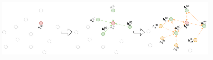
— DGL docs
Take a look at the DGL mini-batch explanation for more details.
In the case of homogeneous graph, target_relation will be
automatically inferred.
The node_features_property parameter must also be sent by the user to specify
where the original node features are saved. Those are needed by the graph neural
networks to compute node embeddings.
All other parameters are optional.
When setting the model parameters, if you specify the split_ratio 1.0, the
model will train normally on a whole dataset without validating its performance
on a validation set. However, if the split_ratio is a value between 0.0 and
1.0 but the graph is too small to have such a split, an exception will be
thrown.
Self-loop edge is added to every node to improve link_prediction
performance if add_self_loop is set to true. Self-loop edges are added
only as edge_type self, not in any other way.
Here is the description of all parameters supported by link prediction that
you can set by calling the set_model_parameters method:
Input:
| Name | Type | Default | Description |
|---|---|---|---|
hidden_features_size | mgp.List[int] | [16, 16] | Defines the size of each hidden layer in the architecture. Input feature size is determined automatically while converting the original graph to the DGL compatible one. |
layer_type | str | graph_attn | Supported values are graph_sage and graph_attn. |
num_epochs | int | 100 | The number of epochs for model training. |
optimizer | str | ADAM | Supported values are ADAM and SGD. |
learning_rate | float | 0.01 | Optimizer’s learning rate. |
split_ratio | float | 0.8 | The split ratio between the training and the validation set. There is no test dataset because it’s assumed that the user first needs to create new edges in the original dataset to test a model on them. |
node_features_property | str | features | Property name where the node features are saved. |
device_type | str | cpu | Defines if the model will be trained using the CPU or Cuda GPU. To run on Cuda GPU, check if the system supports it with torch.cuda.is_available(), then set this flag to cuda. |
console_log_freq | int | 5 | Specifies how often results will be printed. This also directly specifies which results will be returned as training and validation results when calling the training method. |
checkpoint_freq | int | 5 | Select the number of epochs on which the model will be saved. The model is persisted on disc. |
aggregator | str | mean | Aggregator used in GraphSAGE model. Supported values are lstm, pool, mean and gcn. |
metrics | mgp.List[str] | [loss, accuracy, auc_score, precision, recall, f1, true_positives, true_negatives, false_positives, false_negatives] | Metrics used to evaluate the training model on the validation set. Additionally, epoch information will always be displayed. |
predictor_type | str | dot | Type of the predictor. A predictor is used for combining node scores to edge scores. Supported values are dot and mlp. |
attn_num_heads | List[int] | [4, 1] | GAT can support the usage of more than one head in each layer except the last one. The size of the list must be the same as the number of layers specified by the hidden_features_size parameter. |
tr_acc_patience | int | 8 | Training patience specifies for how many epochs drop in accuracy on the validation set is tolerated before the training is stopped. |
context_save_dir | str | None | Path where the model and predictor will be saved every checkpoint_freq epochs. |
target_relation | str | None | Unique edge type used for training. Users can provide only edge_type or tuple of the source node, edge type, dest_node if the same edge_type is used with more source-destination node combinations. |
num_neg_per_pos_edge | int | 1 | Number of negative edges that will be sampled per one positive edge in the mini-batch training. |
batch_size | int | 256 | Batch size used in both training and validation procedure. It specifies the number of indexes in each batch. |
sampling_workers | int | 5 | Number of workers that will cooperate in the sampling procedure in the training and validation. |
last_activation_function | str | sigmoid | Activation function that is applied after the last layer in the model and before the predictor_type. Currently, only sigmoid is supported. |
add_reverse_edges | bool | False | Whether the module should add reverse edges for each existing edge in the obtained graph. If the source and destination node are of the same type, edges of the same edge type will be created. If the source and destination nodes are different, then the prefix rev_ will be added to the previous edge type. Reverse edges will be excluded as message passing edges for corresponding supervision edges. |
add_self_loop | bool | False | Flag which specifies whether self loop edges will be added to every node in the graph with edge_type set to “self”. |
Output:
status: bool->Trueif all parameters were successfully updated,Falseotherwise.message: str->OKif all parameters were successfully updated,Error messageotherwise.
Usage:
When calling the procedure, send only those parameters that need changing from their default values:
CALL link_prediction.set_model_parameters({num_epochs: 100, node_features_property: "features", tr_acc_patience: 8, target_relation: "CITES", batch_size: 256, last_activation_function: "sigmoid", add_reverse_edges: True})
YIELD status, message
RETURN status, message;
train()
The train procedure is used to train a model and it doesn’t take any input parameters.
Input:
subgraph: Graph(OPTIONAL) ➡ A specific subgraph, which is an object of type Graph returned by theproject()function, on which the algorithm is run. If subgraph is not specified, the algorithm is computed on the entire graph by default.
Output:
training_results: List[Dict[str, float]]-> List of training results through epochs. Model’s performance is evaluated everyconsole_log_freqepochs.validation results: List[Dict[str, float]]-> List of validation results through epochs. Model’s performance is evaluated everyconsole_log_freqepochs.
Usage:
To train the module and get the training and validation results summarized through epochs, use the following query:
CALL link_prediction.train()
YIELD training_results, validation_results
RETURN training_results, validation_results;
get_training_results()
The get_training_results() procedure is used to get performance data obtained
from the last training. The results are in the same format as the results of the
train() procedure. If there is no loaded model, an exception will be thrown.
Input:
subgraph: Graph(OPTIONAL) ➡ A specific subgraph, which is an object of type Graph returned by theproject()function, on which the algorithm is run. If subgraph is not specified, the algorithm is computed on the entire graph by default.
Output:
training_results: List[Dict[str, float]]-> List of training results through epochs. Model’s performance is evaluated everyconsole_log_freqepochs.validation results: List[Dict[str, float]]-> List of validation results through epochs. Model’s performance is evaluated everyconsole_log_freqepochs.
Usage:
To get the performance data from the last training, use the following query:
CALL link_prediction.get_training_results()
YIELD training_results, validation_results;
RETURN training_results, validation_results;
predict()
The predict() procedure takes two arguments, src_vertex and dest_vertex,
and predicts whether there is an edge between them or not. It supports an
“actual” prediction scenario when the edge doesn’t exist and the user wants to
predict whether there is an edge or not but also a scenario in which there is an
edge between two vertices and the user wants to check the model’s evaluation.
Input:
-
subgraph: Graph(OPTIONAL) ➡ A specific subgraph, which is an object of type Graph returned by theproject()function, on which the algorithm is run. If subgraph is not specified, the algorithm is computed on the entire graph by default. -
src_vertex: mgp.Vertex-> Source vertex of the edge. -
dest_vertex: mgp.Vertex-> Destination vertex of the edge.
Output:
score: mgp.Number-> Score between 0 and 1 that represents the probability of two nodes being connected.
Usage:
To get a prediction about an existence of a relationship, use the following query:
MATCH (v1:PAPER {id: "ID_1"})
MATCH (v2:PAPER {id: "ID_2"})
CALL link_prediction.predict(v1, v2)
YIELD score
RETURN score;
recommend()
The recommend() procedure can be used to recommend the best k nodes from
dest_vertices to src_vertex. It is implemented efficiently using the max
heap data structure. The best nodes are determined based on the edge scores.
Metrics specific to recommendation systems (precision@k, recall@k, f1@k and
average precision) are logged to the standard output. K is equal to
the given min(k, length(dest_vertices), length(results)) where results are a
list of all recommendations given by the model(classified as a positive
example.)
Input:
-
subgraph: Graph(OPTIONAL) ➡ A specific subgraph, which is an object of type Graph returned by theproject()function, on which the algorithm is run. If subgraph is not specified, the algorithm is computed on the entire graph by default. -
src_vertex: mgp.Vertex→ Source node. -
dest_vertices: List[mgp.Vertex]→ Destination nodes. If they are not of the same type, an exception is thrown. -
k: int→ Number of edges to recommend.
Output:
score: mgp.Number→ Score between 0 and 1 that represents the probability of two nodes being connected.recommendation: mgp.Vertex→ A reference to the target node.
Usage:
To get the k-nodes recommendations, use the following query:
MATCH (v1:Customer {id: "8779-QRDMV"})
MATCH (p:Plan)
WITH collect(p) AS all_plans, v1
CALL link_prediction.recommend(v1, all_plans, 5)
YIELD score, recommendation
RETURN v1, score, recommendation;
load_context()
Loading the context means loading the model and the predictor. If the user specifies the path, the method will try to load it from there. Otherwise, context will be loaded from the default parameter specified in the link_prediction_parameters module.
Input:
-
subgraph: Graph(OPTIONAL) ➡ A specific subgraph, which is an object of type Graph returned by theproject()function, on which the algorithm is run. If subgraph is not specified, the algorithm is computed on the entire graph by default. -
path: str→ Path to the folder where the model and the predictor are saved.
Output:
status: mgp.Any→ True to indicate that execution went well.
Usage:
To load the context, use the following query:
CALL link_prediction.load_context()
YIELD status
RETURN status;
reset_parameters()
You can explicitly reset parameters whenever you want. Note, however, that parameters will be reset before the training even if not specified because of implementation reasons.
Input:
subgraph: Graph(OPTIONAL) ➡ A specific subgraph, which is an object of type Graph returned by theproject()function, on which the algorithm is run. If subgraph is not specified, the algorithm is computed on the entire graph by default.
Output:
status: mgp.Any→ True to indicate that method is successfully finished.
Usage:
To reset the parameters, use the following query:
CALL link_prediction.reset_parameters()
YIELD status
RETURN status;
Benchmarks
Memgraph extensively tested the model on the CORA dataset and the Telecom recommendation dataset. To show you how the training performance could progress through epochs, here are the results for one of our basic models tried on the Cora dataset:
| epoch_num | AUC | accuracy | precision | recall | f1 |
|---|---|---|---|---|---|
| 1 | 0.64 | 0.594 | 0.613 | 0.494 | 0.547 |
| 2 | 0.781 | 0.696 | 0.711 | 0.663 | 0.686 |
| 3 | 0.798 | 0.729 | 0.752 | 0.682 | 0.715 |
| 4 | 0.754 | 0.686 | 0.716 | 0.617 | 0.663 |
| 5 | 0.789 | 0.711 | 0.715 | 0.7 | 0.707 |
| 6 | 0.813 | 0.756 | 0.742 | 0.784 | 0.763 |
| 7 | 0.884 | 0.772 | 0.764 | 0.791 | 0.775 |
| 8 | 0.859 | 0.775 | 0.781 | 0.766 | 0.773 |
| 9 | 0.871 | 0.805 | 0.822 | 0.777 | 0.798 |
| 10 | 0.832 | 0.759 | 0.776 | 0.729 | 0.752 |
Example
Database state
The database contains the following data:
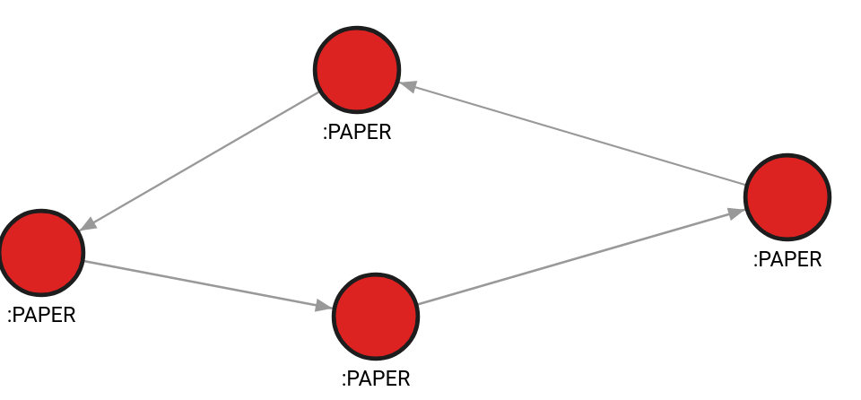
Created with the following Cypher queries:
CREATE (v1:PAPER {id: 10, features: [1, 2, 3]});
CREATE (v2:PAPER {id: 11, features: [1.54, 0.3, 1.78]});
CREATE (v3:PAPER {id: 12, features: [0.5, 1, 4.5]});
CREATE (v4:PAPER {id: 13, features: [0.78, 0.234, 1.2]});
MATCH (v1:PAPER {id: 10}), (v2:PAPER {id: 11}) CREATE (v1)-[e:CITES {}]->(v2);
MATCH (v2:PAPER {id: 11}), (v3:PAPER {id: 12}) CREATE (v2)-[e:CITES {}]->(v3);
MATCH (v3:PAPER {id: 12}), (v4:PAPER {id: 13}) CREATE (v3)-[e:CITES {}]->(v4);
MATCH (v4:PAPER {id: 13}), (v1:PAPER {id: 10}) CREATE (v4)-[e:CITES {}]->(v1);
Set model parameters
To set the model parameters, use the following query:
CALL link_prediction.set_model_parameters({target_relation: ["PAPER", "CITES", "PAPER"], node_features_property: "features",
split_ratio: 1.0, predictor_type: "mlp", num_epochs: 100, hidden_features_size: [256], attn_num_heads: [1]})
YIELD status, message
RETURN status, message;
Train the module
To train the module, use the following query:
CALL link_prediction.train() YIELD training_results, validation_results
RETURN training_results, validation_results;
Train results:
+--------------------+--------------------+--------------------+--------------------+--------------------+
| epoch_num          | accuracy           | auc_score          | loss               | precision          |
+--------------------+--------------------+--------------------+--------------------+--------------------+
| 17                 | 0.833              | 0.906              | 0.428              | 1.0                |
| 18                 | 0.917              | 0.938              | 0.393              | 1.0                |
| 19                 | 0.833              | 0.938              | 0.365              | 0.75               |
| 20                 | 0.917              | 0.938              | 0.341              | 1.0                |
| 21                 | 0.917              | 0.938              | 0.315              | 1.0                |
| 22                 | 0.833              | 0.969              | 0.296              | 0.75               |
| 23                 | 0.917              | 1.0                | 0.277              | 1.0                |
| 24                 | 0.917              | 1.0                | 0.246              | 0.8                |
| 25                 | 0.917              | 1.0                | 0.233              | 0.8                |
| 26                 | 1.0                | 1.0                | 0.202              | 1.0                |
Predict relationships
To predict relationships, use the following query:
MATCH (v1:PAPER {id: 10})
MATCH (v2:PAPER {id: 12})
CALL link_prediction.predict(v1, v2)
YIELD score
RETURN score;
Result:
+-------+
| score |
| 0.104 |
FAQ
Why can I get into problems with reverse edges?
Having a reverse_edge in your dataset can be a problem if they are not
excluded from message passing edges in the prediction of its opposite edge(supervision edge). The best thing you can do is have a directed graph
and the module will automatically add reverse edges, if you specify
add_reverse_edges in the set_model_parameters method, in a way that doesn’t
cause information flow.
What is a transductive dataset split?
The transductive dataset split assumes that the entire graph can be observed in
all dataset splits. We distinguish four types of edges, and those are:
validation, training, message passing and supervision edges.
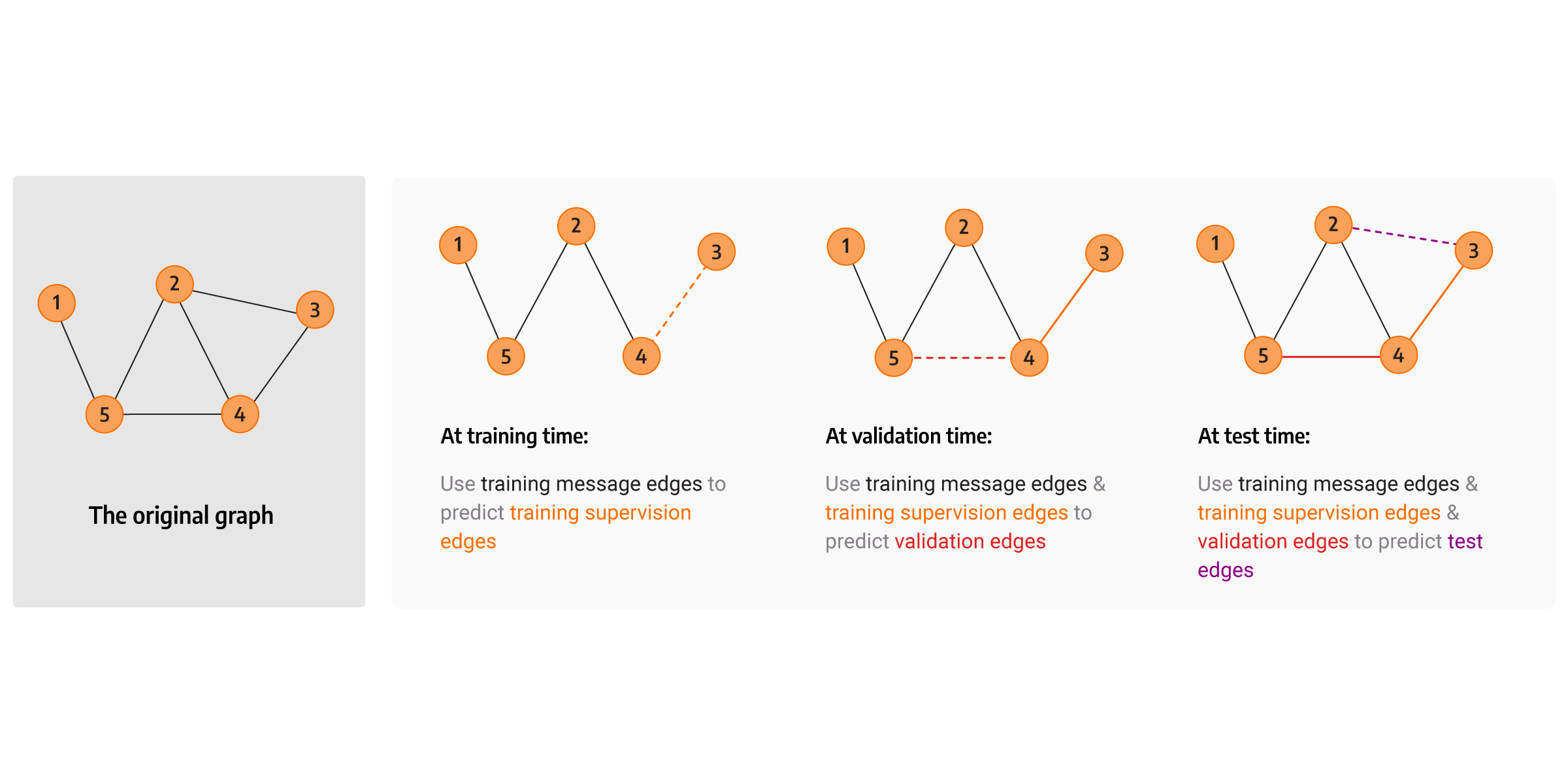
The transductive dataset split is described in detail by prof. Jure Leskovec at one of its presentations for Graph ML course.