
Graph Search Algorithms: Developer's Guide
Graph search algorithms form the backbone of many applications, from social network analysis and route planning to data mining and recommendation systems. In this developer's guide, we will delve into the world of graph search algorithms, exploring their definition, significance, and practical applications.
At its core, a graph search algorithm is a technique used to traverse a graph, which is a collection of nodes connected by relationships. In various domains such as social networks, web pages, or biological networks, graph theory offers a powerful way to model complex interconnections.
The significance of graph search algorithms lies in their ability to efficiently explore and navigate these intricate networks. By traversing the graph, these algorithms can uncover hidden patterns, discover the shortest paths, and identify clusters.
One of the primary benefits of graph search algorithms is their adaptability to a wide array of applications. Whether you're developing a social media platform, designing a logistics system, or building a recommendation engine, by understanding the foundations of graph search algorithms and learning how to leverage them effectively, you'll unlock new possibilities for solving complex problems and advancing your development skills.
Types of graphs
Graphs are versatile data structures that can represent various types of relationships between objects. Understanding the different types of graphs is essential for effectively applying graph search algorithms. In this chapter, we will explore the most common types of graphs, their characteristics, and applications, along with visual examples to aid comprehension.
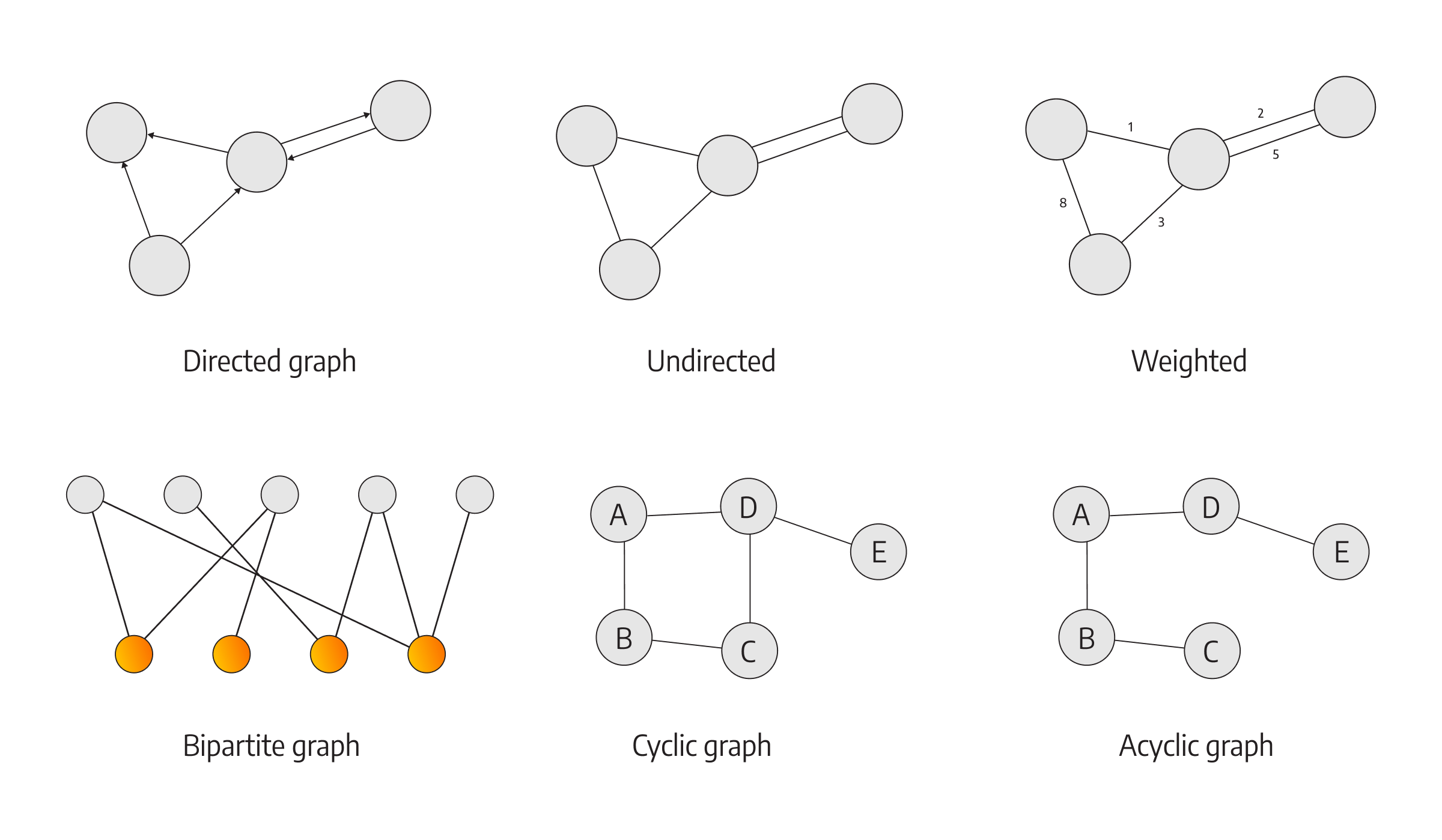
Directed graphs, also known as a digraph, consist of nodes connected by directed relationships. In a directed relationship, there is a specific direction from one node (the source) to another node (the target). A directed graph is used to model relationships with a sense of direction, such as web pages with hyperlinks, dependencies between tasks, or social media following relationships.
Undirected graph is a graph in which relationships have no specified direction. Undirected graphs are commonly used to represent relationships that are bidirectional, such as friendships in a social network or connections between web pages.
Weighted graphs assign numerical values, known as weights, to relationships to represent the strength, distance, or cost between nodes. These weights can influence the behavior of graph search algorithms, allowing for more specific optimizations or finding the shortest or cheapest paths. Weighted graphs find applications in areas like network routing, resource allocation, or finding optimal solutions in various domains.
Bipartite graph is a graph whose nodes can be divided into two disjoint sets, and all relationships connect nodes from different sets. Bipartite graphs are often used to model relationships between two distinct types of entities, such as users and products, students and courses, or employees and skills. They are particularly useful in applications like recommendation systems or matching problems.
Cyclic graphs contain at least one cycle, which is a path that starts and ends at the same node. Acyclic graphs, as the name suggests, do not contain any cycles. Cyclic graphs can represent scenarios with repeating or circular relationships, while acyclic graphs are often used in tasks like topological sorting or modeling hierarchical structures.
Understanding the different types of graphs provides developers with a foundation for choosing the appropriate graph representation for their specific problem. Each type has its own characteristics and applications, and selecting the right graph structure can significantly impact the efficiency and accuracy of graph search algorithms.
Basic graph search algorithms
In the realm of graph search algorithms, two fundamental techniques stand out: Breadth-first search (BFS) and Depth-first search (DFS). These algorithms provide crucial building blocks for traversing and exploring graphs in different ways. While BFS focuses on exploring the breadth of a graph by systematically visiting all neighboring nodes before moving deeper, DFS delves into the depths of a graph, exhaustively exploring one branch before backtracking.
BFS and DFS Basics
Depth-first search is an algorithm that explores a graph by traversing as far as possible along each branch before backtracking. The key working principle of DFS is to visit a node and then recursively explore its unvisited neighbors until there are no more unvisited nodes in that branch. This depth-first exploration strategy can be implemented using a stack or recursion. By utilizing a stack, DFS ensures that the most recently discovered nodes are visited first, delving deeper into the graph.
Breadth-first search or the BFS algorithm systematically explores a graph by visiting all the neighboring nodes of a given level before moving to the next level. The core working principle of BFS is to use a queue to maintain a level-wise exploration order. Initially, the algorithm starts with a source node, enqueues its neighbors, and continues this process until all nodes have been visited. The breadth-first traversal strategy ensures that nodes are visited in increasing order of their distance from the source, allowing for finding the shortest path in unweighted graphs.
Both DFS and BFS maintain a record of visited nodes to prevent revisiting the same node repeatedly. This visited node management is crucial to ensure that the algorithms terminate correctly and avoid infinite loops in cyclic graphs. Typically, a boolean array or hash set is used to keep track of visited nodes, marking them as visited when they are encountered during graph traversal.
In terms of time and space complexities, the time complexity of both algorithms is O(V + E), where V represents the number of vertices (nodes) and E represents the number of edges (relationships) in the graph. The space complexity for both algorithms is O(V) since DFS requires a stack to keep track of nodes, while BFS requires a queue to store nodes during traversal.
Use cases
DFS and BFS are powerful graph search algorithms that find wide-ranging applications across various domains.
BFS is often employed in web crawling, where it helps in systematically exploring and indexing web pages starting from a given source page. By utilizing BFS, web crawlers can visit neighboring pages before moving to deeper levels, ensuring comprehensive coverage of a website or a set of interconnected websites. BFS-based crawling allows search engines to index web pages efficiently, enabling users to find relevant information quickly.
BFS plays a vital role in route planning algorithms, especially in unweighted graphs or maps. It helps in finding the shortest path between two locations, ensuring that the traversal explores neighboring locations before expanding the search to farther areas. By utilizing BFS, route planning applications can provide optimal directions, whether it's for driving, walking, or public transportation.
DFS and BFS are valuable tools in recommendation engines, helping to discover relevant content or items for users. DFS can be used to find similar users or items based on shared characteristics, facilitating collaborative filtering approaches. BFS can explore the graph of user-item interactions to recommend items that are highly connected or related to the user's preferences.
In social networks DFS can be used to identify connected components, finding groups of individuals who are mutually connected. BFS is useful for determining the shortest path between two individuals, showcasing the most efficient connections within the network. These algorithms also aid in social network analysis, such as identifying influential individuals or detecting communities and clusters.
The applications mentioned above provide just a glimpse into the broad spectrum of possibilities that DFS and BFS offer. These algorithms are versatile tools that can be adapted to various domains and problem spaces, allowing developers to tackle complex challenges efficiently.
Implementation
Implementing DFS and BFS requires careful consideration and adherence to best practices to ensure correct and efficient implementations.
As a first step, understand the implications of DFS and BFS traversal orders and select the appropriate order for your specific use case.
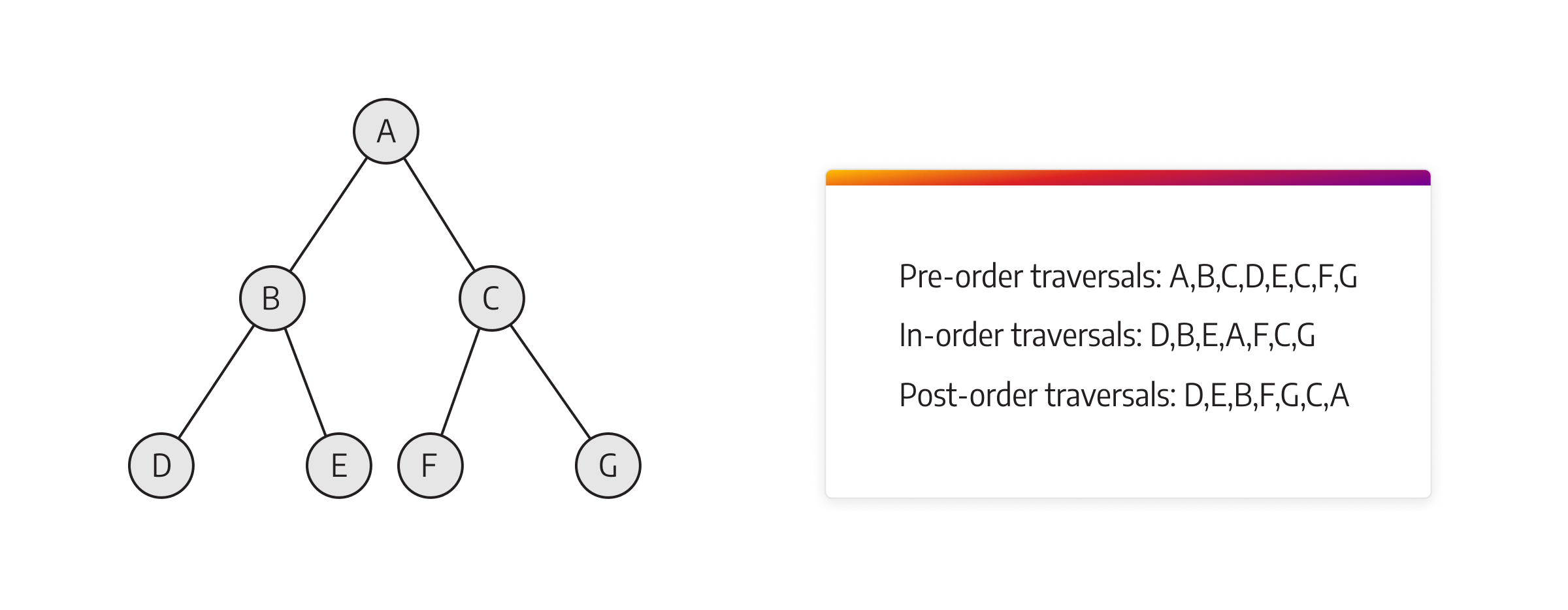
For DFS, decide whether to explore the graph in a pre-order, in-order, or post-order manner. In pre-order DFS, a node is processed (visited or printed) before traversing its children. The traversal starts at the root node and then recursively explores the left and right subtrees in pre-order. The pre-order strategy is often used in tree-based traversals.
In in-order DFS, a node is processed between the traversal of its left and right subtrees. In other words, the left subtree is explored first, followed by processing the current node and then exploring the right subtree. In-order DFS is primarily used in binary tree traversals and is especially relevant for binary search trees to visit nodes in ascending order. In post-order DFS, a node is processed after traversing its children.
The traversal starts at the root node and recursively explores the left and right subtrees in post-order before finally processing the current node. Post-order DFS is commonly used in tree-based algorithms that require processing child nodes before processing the parent node.
Pre-order is often useful for constructing a copy of the tree or encoding the tree structure. In-order is suitable for tasks like sorting elements in a binary search tree. Post-order is valuable for tasks such as calculating expressions in a parse tree.
For BFS, ensure that the traversal explores nodes in the order dictated by the queue, maintaining the level-wise exploration.
If the graph contains cycles, consider incorporating cycle detection mechanisms or break conditions to avoid infinite loops during traversal. Implement a mechanism to handle backtracking in DFS to ensure that previously visited nodes are not revisited unnecessarily.
Be aware of the time and space complexities of DFS and BFS to gauge their efficiency and performance for different graph sizes and structures.
Consider the following pseudocode examples for implementing DFS and BFS.
Depth-First Search (DFS):
function dfs(graph, start):

    stack.push(start)

    visited[start] = true


    while stack is not empty:

        current = stack.pop()

        process(current)


        for each neighbor in graph.adjacentNodes(current):

            if neighbor is not visited:

                stack.push(neighbor)

                visited[neighbor] = true
BFS (Breadth-First Search):
function bfs(graph, start):

    queue.enqueue(start)

    visited[start] = true


    while queue is not empty:

        current = queue.dequeue()

        process(current)


        for each neighbor in graph.adjacentNodes(current):

            if neighbor is not visited:

                queue.enqueue(neighbor)

                visited[neighbor] = true
Advanced graph search algorithm
In addition to the basic graph search algorithms DFS and BFS, advanced graph search algorithms offer powerful solutions to more complex problems. Two such algorithms, Dijkstra's and Bellman-Ford algorithms, play a crucial role in finding the shortest paths in weighted graphs. In this section, we will introduce Dijkstra's Algorithm and Bellman-Ford Algorithm, highlighting their significance in optimizing route planning, network routing, and other applications that involve finding the most efficient paths in graphs with weighted edges.
Check out our Graph algorithms infographic for a visual overview of these and other advanced algorithms available in Memgraph.
Dijkstra's and Bellman-Ford basics
Dijkstra's algorithm is a widely used algorithm for finding the shortest path between a source node and all other nodes in a weighted graph. It works on graphs with non-negative relationship weights and is particularly suitable for scenarios like route planning, network routing, or finding optimal paths in transportation networks.
Dijkstra's algorithm employs a greedy approach, iteratively selecting the node with the smallest tentative distance and updating the distances of its neighboring nodes until all nodes have been visited. It maintains a priority queue or a min-heap to efficiently extract the node with the minimum distance. It has a time complexity of O(V^2) using the adjacency matrix representation of the graph. The time complexity can be reduced to O((V+E)logV) using an adjacency list representation of the graph, where E is the number of edges (relationships) in the graph and V is the number of vertices (nodes) in the graph.
Bellman-Ford is another important algorithm for finding the shortest paths in graphs that may contain negative relationship weights. Unlike Dijkstra's algorithm, which assumes non-negative weights, the Bellman-Ford algorithm can handle graphs with negative weights as long as there are no negative cycles. It is commonly used in scenarios such as network routing, distance vector routing protocols, or detecting negative cycles in graphs. The Bellman-Ford algorithm iterates through all relationships in the graph repeatedly, updating the distances of nodes based on the relaxation principle. It maintains an array to track the distances of nodes and iterates through all relationships |V| - 1 times to ensure convergence. The time complexity of the Bellman-Ford algorithm is O(V E), where V represents the number of vertices and E represents the number of relationships in the graph.
Use cases
Dijkstra's and Bellman-Ford algorithms excel in solving real-world problems related to route planning, network optimization, resource allocation, and various other domains.
Both algorithms are extensively used in route planning applications to find the shortest path between locations in transportation networks, such as roads, railways, or flight routes. These algorithms enable navigation systems to calculate optimal routes for drivers, public transportation, and logistics planning.
In computer networks, these graph search algorithms play a crucial role in determining the most efficient paths for routing packets or establishing network connections. They help optimize the flow of data, reduce latency, and improve network performance. Dijkstra's Algorithm is commonly used in link-state routing protocols like OSPF (Open Shortest Path First), while the Bellman-Ford algorithm is employed in distance-vector routing protocols like RIP (Routing Information Protocol).
Both Dijkstra's algorithm and Bellman-Ford algorithm find applications in resource allocation problems, such as allocating resources in cloud computing, scheduling tasks, or optimizing supply chains. These algorithms assist in identifying the most cost-effective or time-efficient paths to allocate resources and optimize resource utilization. The Bellman-Ford algorithm is especially useful with negative relationship weights (without negative cycles) in scenarios where resource costs or constraints are involved.
The algorithms also aid in managing critical infrastructure and facilities, such as power grids, telecommunications networks, or water distribution systems where they can identifying optimal paths for maintenance crews, detecting faults or disruptions, and optimizing resource allocation for efficient operation.
They can also help optimize supply chain and logistics operations, such as inventory management, order fulfillment, or delivery route optimization by determining the most efficient paths for transporting goods, minimizing costs, and improving customer satisfaction.
The applications mentioned above are just a glimpse of the diverse possibilities that Dijkstra's and Bellman-Ford algorithms offer. Both are versatile and can be adapted to various problem domains requiring optimization and efficient path-finding in graphs.
Implementation
When implementing graph search algorithms, such as Dijkstra's algorithm and Bellman-Ford algorithm, be sure to provide proper handling of relationship weights according to the requirements of the algorithms.
In the case of using Dijkstra's algorithm, validate that the relationship weights are non-negative. For the Bellman-Ford algorithm, ensure that the graph does not contain any negative cycles to maintain correct behavior.
Initialize data structures and variables appropriately before starting the algorithm. Set initial distances to infinity for Dijkstra's algorithm and initialize distances to 0 for the source node in the Bellman-Ford algorithm. Initialize other auxiliary data structures as required, such as priority queues or arrays.
Understand the relaxation step in each algorithm and implement it correctly. Update the distances and other relevant information whenever a shorter path is found during the traversal.
Implement appropriate termination conditions for the algorithms to ensure they terminate correctly. For Dijkstra's algorithm, terminate when the destination node is reached or when all reachable nodes have been visited. In the Bellman-Ford algorithm, terminate when no further updates can be made, indicating that the distances have converged.
Consider the following pseudocode examples for implementing Dijkstra's and Bellman-Ford algorithms. The pseudocode assumes the existence of appropriate data structures like priorityQueue for Dijkstra's Algorithm and arrays like distances and visited to store necessary information.
Dijkstra's algorithm:
function dijkstra(graph, start):

    distances[start] = 0

    priorityQueue.enqueue(start, 0)


    while priorityQueue is not empty:

        current = priorityQueue.dequeue()

        visited[current] = true


        for each neighbor in graph.adjacentNodes(current):

            if not visited[neighbor]:

                distance = distances[current] + graph.edgeWeight(current, neighbor)

                if distance < distances[neighbor]:

                    distances[neighbor] = distance

                    priorityQueue.enqueue(neighbor, distance)
Bellman-Ford algorithm:
function bellmanFord(graph, start):

    distances[start] = 0


    for i = 1 to |V| - 1:

        for each edge in graph.edges:

            source = edge.source

            destination = edge.destination

            weight = edge.weight


            if distances[source] + weight < distances[destination]:

                distances[destination] = distances[source] + weight


    for each edge in graph.edges:

        source = edge.source

        destination = edge.destination

        weight = edge.weight


        if distances[source] + weight < distances[destination]:

            // Negative cycle detected

            // Handle the presence of negative cycles accordingly
Performance analysis and optimization
Efficient performance is crucial when working with graph search algorithms to tackle real-world problems effectively. The increase in the number of nodes and relationships in the graph and the higher density of the graph affect the algorithm's performance.
Efficiency can be increased by incorporating domain-specific knowledge or rules, thus heuristically guiding the search process towards more promising paths and prioritizing nodes or edges, improving efficiency. Another way is by pruning, or eliminating branches or subtrees from further exploration based on certain criteria. Pruning techniques, such as alpha-beta pruning in game-playing scenarios, discard portions of the search space that are deemed irrelevant, significantly reducing the algorithm's runtime. Another technique is memoization, which involves storing previously computed results to avoid redundant calculations. In graph search algorithms, memoization can cache intermediate results, such as computed distances or paths, to avoid re-computation, especially when there are overlapping subproblems.
BFS and DFS can benefit from performance optimizations by applying pruning techniques to skip unnecessary relationships or paths during traversal. Additionally, using appropriate data structures for maintaining visited nodes and tracking the traversal order can improve efficiency.
The performance of Dijkstra's algorithm can be optimized by utilizing efficient data structures like priority queues or heaps to retrieve nodes with the minimum distance more quickly. Heuristics can also be incorporated to prioritize the exploration of nodes that are more likely to yield shorter paths.
The Bellman-Ford algorithm can benefit from early termination if no updates are made during an iteration, indicating that the distances have converged. This can save unnecessary iterations, improving runtime.
Wrap up
In this comprehensive guide, we have explored the fundamental concepts and practical applications of various graph search algorithms. Starting with the basic algorithms like BFS and DFS, we gained insights into their working principles and traversal strategies. We also delved into Dijkstra's and Bellman-Ford algorithms, which excel in solving complex problems involving weighted graphs. We explored their specific use cases, advantages over basic algorithms, and discussed optimization techniques to improve their efficiency.
Understanding the nuances of graph search algorithms empowers the developer community to solve a wide range of problems across diverse domains, ultimately contributing to the advancement of technology and society.
If you want to know more about various graph algorithms, download the Graph Algorithms for Beginners whitepaper that also deals with centrality and machine learning algorithms.