Diving Into the Vehicle Routing Problem

Introduction

Your small healthy food-producing company is doing really well this season. Having an established line of customers throughout the year is driving the business stable and products are delivered to them without any delays. Your route for every customer is planned in advance, depending on the number of workers with pick-up cars who deliver the food.

However, the summer season is approaching, and soon a lot of temporary seasonal customers are going to be ad hoc ordering healthy meals from your company. Suddenly the logistics are hectic and the routes are impossible to plan since the orders are coming in dynamically and stochastically. New suboptimal routes together with fuel costs are cutting the company's growth process and revenue, and you need to come up with a solution about how to organize your pick-up vehicles better.

Luckily, this kind of problem is well known in optimization theory and it's called Vehicle Routing Problem. In this article, you'll learn more about the variations of the problem, how to model synthetic data to prepare for real-world scenarios, and of course, possible approaches for the solution.

Defining the problem

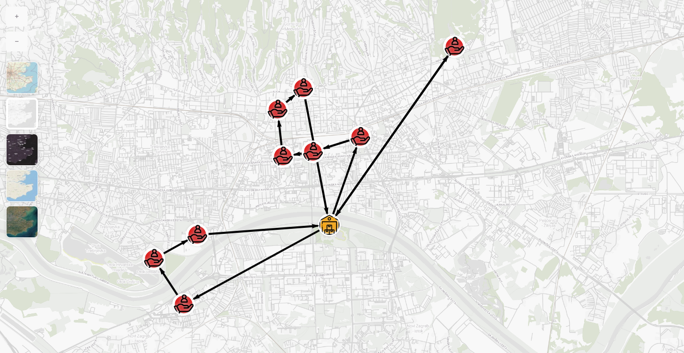
We can think of VRP as a generalization of TSP (Traveling Salesperson Problem), with additional entities, i.e. vehicles in this case. In the classic TSP, the salesperson must visit all the customers once and return to the starting position with a minimized route cost, while in VRP a fleet of vehicles is used in order to do the same. They usually start from the same spot which can represent a depot of production. The problem itself is NP-hard and therefore advises heuristics, approximation algorithms, or numerical optimization in order to reach a feasible solution.

VRP has many variations of its problem and the main distinctions come with respect to the known information at the beginning. The basic one is called static VRP and this means that all the information about the locations of the customers, and their requests are known in advance. The advantage of getting to know all the information ultimately yields better results with shorter vehicle lengths passed, however, it doesn’t truly depict a real-world scenario.

The more representative use case would be the Dynamic Vehicle Routing Problem (DVRP) which is featured by having at least one of its parameters time-dependent. Most commonly, that would be the arrival time of the request itself, making it unknown to the user when a certain immediate customer demand would need to be served. The end result would then be a feasible adaptation of the initially constructed routes.

VRP can be modeled in additional ways in order to make it look more realistic. Most certainly one would want to work with time windows, and the problem would then be known as Dynamic Vehicle Routing Problem with Time Windows (DVRPTW). The time windows themselves symbolize the opening and closing hours of the service that ordered the product from the distribution company. If we define the reaction time as the time needed in the final solution from request arrival to service delivery finish, the solution goal would be minimizing reaction time with respect to service opening hours, as well as the initial one of minimizing the route length. Additional penalties can be introduced if service hours are not met.

Modeling the data

One of the important things to verify the VRP solution is applying it to concrete data. Although there are a lot of open datasets online, the number of requests or degree of dynamism can strongly differ. The DIY approach would include distributing the arrival of immediate requests by the Poisson process since it is particularly used for modeling the rate that something occurs in a random manner. Location of the customers don’t actually have a particular distribution they are subordinate to, therefore a uniform distribution would suffice. The same goes for service opening and closing hours as well.

Modeling the problem

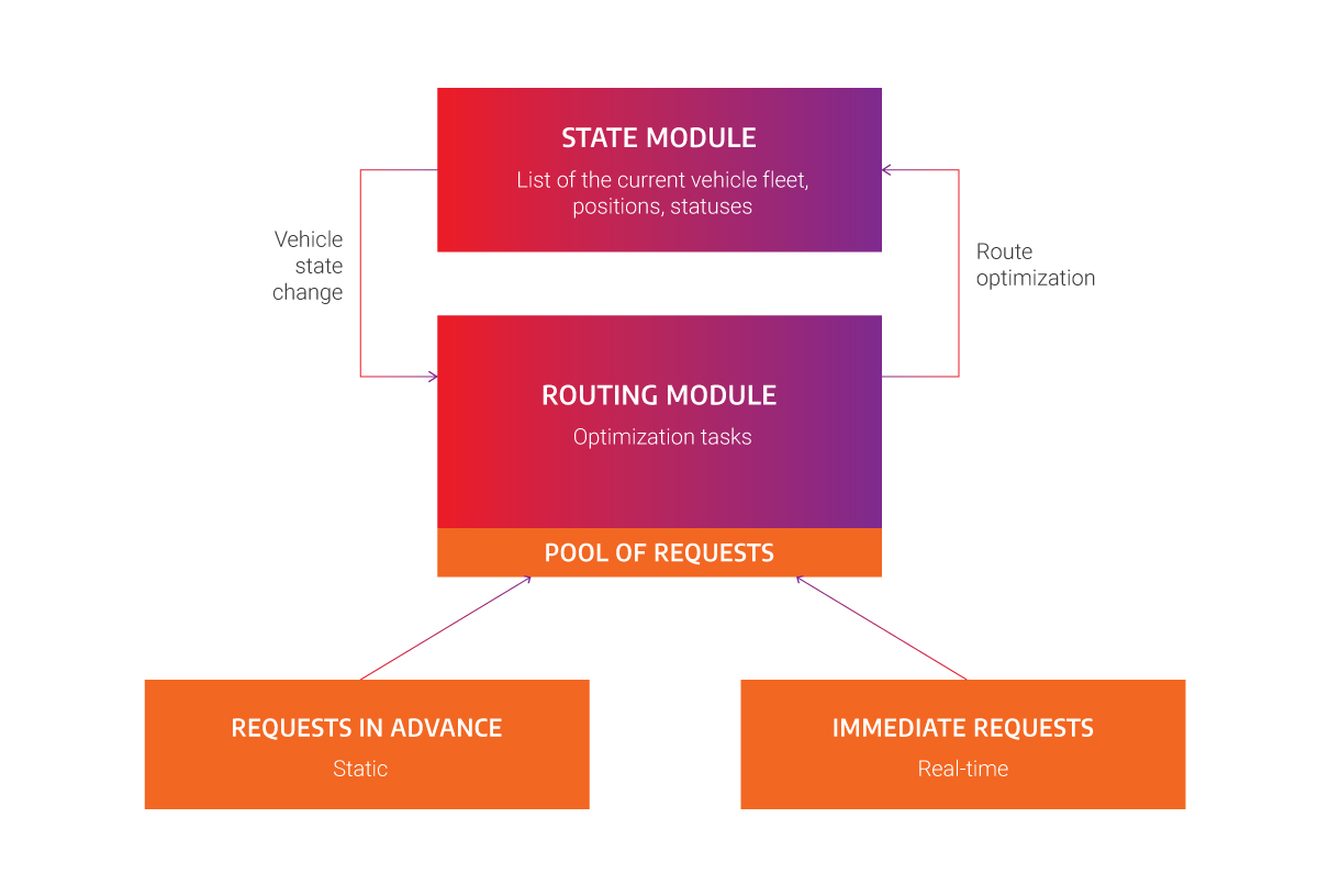
Until now we have just been adding features to our routing problem, it’s time to model the state itself to ensure the validity of every step throughout routing and re-routing the vehicles. The state with 2 modules, one representing the vehicle's information at a certain point in time, and the other representing a request pool that would serve as a routing module.

Vehicle state module

To precisely gain information about every vehicle in real-time, one would need several parameters for doing so. One of them would definitely be the location of the vehicle on the map, e.g. latitude and longitude or some other one in a different coordinate system. If the vehicle is having a finite amount of products in its trunk, one might add a capacity that might decrease with every request served, after which the vehicle needs to turn back to its depot for replenishing. That doesn’t need to be the case if, for example, the vehicle represents repairmen helping customers in need. The final parameter for modeling a basic vehicle state would be the current action the vehicle is performing – idle, driving (to a specific customer or going back to depot), and serving the customer.

Routing module

The routing module consists of a pool of incoming requests. In the beginning, there are only requests known in advance in the pool, which is being increased with immediate requests as time goes by and decreases with requests served over time.

Events and rerouting

From the 2 modules, we can distinguish 2 types of events – a vehicle state change event, occurring if a particular vehicle changed its state, and request event, occurring when a new request appeared.

The vehicle state change event would occur for example if the vehicle changed its coordinates, changed the action it is currently doing, or changed its capacity in the trunk. It does not require rerouting, however, that is triggered by a request event. Since a customer would need to be informed as fast as possible what would be a possible time for delivery, the route would need to be adapted in the most feasible way.

Another thing to take into consideration is some hard constraints that need to be satisfied throughout the delivery. All the served requests in the solution have to stay in place, as going back in time is not “yet” possible. As for service opening hours, one can have soft or hard demands about meeting them, and sometimes the evaluation of the solution is modeled that slight delays do not affect the solution that much.

Possible approaches

The static vehicle routing problem has been already investigated in the late '70s, where Solomon [1] proposed an insertion heuristic of handling VRPTW. The insertion bases itself around minimizing the total delay on each customer request. However, in the case of streaming requests, one might find different approaches in scheduling further requests, so here are a few of them, described in another paper [2]:

• Nearest neighbor (NN) - out of all the remaining requests, always move to the nearest neighbor for every vehicle
• First come, first served (FCFS) - schedule requests based on the request arrival time
• Partitioning policy (PART) - the map is divided into subregions, in which the requests are taken in the FCFS order
• Stochastic Queue Median (SQM) - after delivering a request, the vehicle moves to the median of the locations of all requests and then proceeds to the next most feasible one

It is easy to see that with more requests coming in at an intense rate, the route will become longer and eventually, suboptimal. However, it is a trade-off in dynamic environments, as the incoming request mostly needs to be processed immediately, so customers can be informed when the order is going to be completed. If the number of immediate requests is too high, one might consider using batching strategies in order to gain more information at the time re-optimization occurs. Most commonly, there are two types of batching strategies:

• Batch strategy by size - Perform routing every M incoming requests
• Batch strategy by time - Perform routing every N minutes

Summary

All things considered, the Vehicle Routing Problem is a very diverse one with respect to its scope and methods of solving, and it is easy to get confused when picking the right algorithm for a specific problem. If you want to check out more about VRP, stay tuned for upcoming blog posts as Memgraph updates its MAGE spells with the purpose of letting developers use the VRP Solver with ease!

If you found this tutorial interesting, you should try out the many other graph analytics algorithms that are part of the MAGE library.

Finally, if you've been working on your own graph algorithms in MAGE and want to share them with developers around the world, have a peek at the contributing guidelines. We'd be more than happy to help you, provide comments and add the module to the MAGE repository.

References:

[1] Solomon, M. (1987). Algorithms for the Vehicle Routing and Scheduling Problems with Time Window Constraints. Oper. Res., 35, 254-265.
[2] Larsen, A. (2000). The dynamic vehicle routing problem. Technical University of Denmark. IMM-PHD No. 2000- 73