Most Common Problems in Energy Management Systems Solved With Graph Analytics

Graph databases are a good choice when dealing with highly connected data in energy management systems. Graph databases are superior compared to relational databases when talking about energy management systems due to their efficient performance, scalability, visualizations and analytics. However, none of these things matter if you can’t answer positively to the single most important question when choosing a technology - is it solving your use case? Because if it isn’t, why even bother with all the non-functional requirements?

For that purpose, here is a list of key questions and problems in the energy network and answers to how graph analytics and algorithms can help detect, prevent and solve them.

Motivation

When dealing with an energy topology, a number of questions rise up that typically don’t exactly correlate with the storage implementation and the query language of relational databases. People in the energy management industry want to find bottlenecks, and hubs, analyze the flow in the network, and find paths between different nodes, while a relational database is only good enough for statistics and aggregate functions. And if your primary use case is aggregating data points and finding insights based on numerical analysis, a relational database might be a good decision. However, a graph database is structure oriented and can answer those truly important questions by traversing the graph to see if certain neighboring nodes fit into different groups, check the connectivity strength among the nodes, etc.

Due to that difference in asking about the structure of entities, rather than only information they hold, graph databases have made Cypher query language to traverse and find patterns and paths along the graph. In the next few sections, we will incorporate some of the basic questions and problems from the energy management systems, and show how graph traversal queries written in Cypher query language, Memgraph’s graph algorithms, and data visualizations in Memgraph Lab might benefit the company and add value in solving these problems.

Example graph

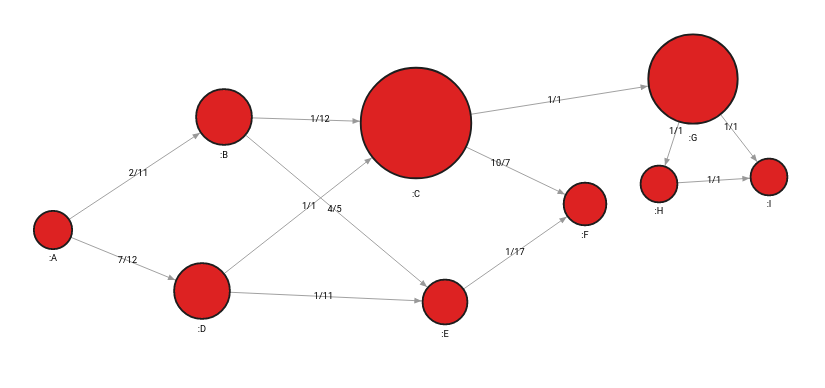
For the purpose of demonstrating traversals and graph algorithms, we will use a simple energy system graph in the image below. The graph below consists of 9 nodes and 12 relationships between them. Additionally, they have the weight and flow properties on each relationship, separated by a dash. Weight and flow properties are used for calculating of shortest paths and flows.

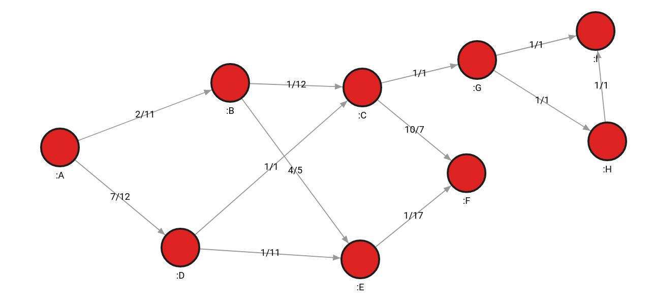
For example, the weight of the relationship between nodes A and B is 2, and the flow is 11.

Finding the path between 2 nodes

Traversing the graph is one of the key benefits of graph databases with a linear time complexity that grows with the number of nodes in the graph. For that purpose, many graph databases leverage graph algorithms that already exist in the mathematical world.

The most common problem concerning pathfinding is how to get the power, or oil, from point A to point B. Most of the time, the goal is to find the shortest distance, but it can also be about using the minimum number of components or avoiding certain country borders. These paths can be found on static data or, more often, dynamical data that changes often. The system needs to find a path quickly and be ready to calculate alternative paths without lag.

In relational databases, designing algorithms for finding shortest paths, such as the Dijkstra’s algorithm for weighted shortest paths, is extremely difficult. However, most graph databases, including Memgraph, include predeveloped pathfinding algorithms that are accessible as a function that is called within the query.

Here is an example of the Dijkstra's algorithm called within a Cypher query:

MATCH p=(n:A)-[r *wShortest (r, n | r.weight)]->(m:F) RETURN p;

The query takes the source node (A) and the target node (F), and returns both the shortest path (the minimum number of hops between nodes) and the least weighted path.

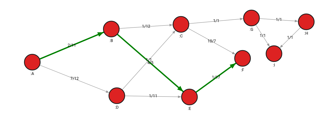
Although both the (A, B, E, F) and (A, D, E, F) paths are the shortest paths, (A, B, E, F) path also weighs less (for example, requires fewer resources). It has a weight of 7, while the (A, D, E, F) path has a weight of 9.

Say that the pipeline between E and F node is blocked, or had a power outage, consequently a raise in the relationship weight by a lot. By rerunning the algorithm, a new path would be found consisting of nodes A, B, C and F with a total weight of 13, thus always using the minimum amount of resources.

In another graph network, it would be beneficial to have all the possible alternative paths between 2 nodes to ensure there are enough viable options for transporting energy. In that case, the ALLSHORTEST algorithm is the most useful one:

MATCH p=(n:A)-[r *ALLSHORTEST (r, n | r.weight)]->(m:F) RETURN p;

Finding weak links and high-risk nodes

When there is a power outage on the field, well-organized companies immediately start fixing the damage, but some households or companies can still be left without power for a considerable amount of time. Sometimes just reacting to damage is not a long-term solution and companies should investigate and predict the behavior of its network and support it with additional or alternative power lines to make the flow of energy consistent and unaffected. Analyzing the network, business, decisions and investments and deciding upon contingency plans or improvements is called risk analytics, and its main goal is to prevent events that lead to unexpected losses.

When one group of nodes is connected to an energy source by only one connection, graph theory refers to that relationship as a bridge. It implies that the graph would be divided into 2 separate networks if the path becomes unusable, causing damage by interrupting the flow of energy going into the secondary component.

To identify bridges in Memgraph, MAGE library includes a special procedure bridges.get():

CALL bridges.get()
YIELD node_from, node_to
MATCH (node_from)-[r]->(node_to)
SET r.bridge = True;

The query identifies the bridge and connects the nodes with an additional relationship to signify that the relationship between the 2 nodes is indeed a bridge.

After inspecting the graph again, we can see that the top part is poorly connected to the rest of the graph, and by disconnecting the relationship, we will get 2 separate components. This might follow a decision to strengthen the poorly connected part and decrease the risk of a power outage.

Another algorithm that can be used to analyze risks and help identify weak points in the topology is betweenness centrality. It measures the extent to which a certain node lies on paths with other nodes. Basically, if a node is connecting more nodes, its betweenness centrality rating is rising. Cutting out nodes with high betweenness centrality might make your network connectivity sparse or possibly disconnect parts of your graph.

Based on the example graph, we can expect that the nodes with the bridge relationship have the highest centrality since the nodes connected with that bridge have a high risk of being disconnected. Indeed, that is what the query below will show:

CALL betweenness_centrality_online.set()
YIELD node, betweenness_centrality
SET node.betweenness_centrality = betweenness_centrality
RETURN node, betweenness_centrality;

Node G got a centrality rating of 0.428 and node C got a centrality rating of 0.6, while, for example, node F got a centrality of 0.047, meaning it’s not of high risk to the topology.

How risk analysis parameters change upon network update

The previous examples showed algorithms that can point out weak points in the topology and urge network support. If the graph is fairly large, it’s not always feasible to recalculate all the algorithms from scratch when data is updated. Some updates are minutely and concern only several nodes, so the whole graph doesn’t need to be recalculated every minute.

Fortunately, a new branch of graph theory involves dynamic graph algorithms, which can calculate the correct outcomes of the traditional graph algorithms based on the local change in the network without recomputing the whole graph.

One of the implementations in Memgraph involves dynamic betweenness centrality, so let's see how it works.

First, a trigger needs to be created, which will dynamically update betweenness centrality after a node or relationship is created or deleted:

CREATE TRIGGER update_bc_trigger
BEFORE COMMIT EXECUTE
  CALL betweenness_centrality_online.update(createdVertices, createdEdges, deletedVertices, deletedEdges)
  YIELD betweenness_centrality, node
  SET node.betweenness_centrality = betweenness_centrality;

Now, let’s modify a graph a bit by adding a few nodes to the secondary component, thus making the risk on nodes G and C even higher:

MATCH (n:I)
MERGE (n)-[:PATH]->(:J)-[:PATH]->(:K)-[:PATH]->(:L)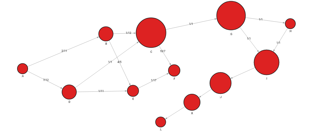

The updated betweenness centrality of node C is 0.579 and that of node G is 0.545, which means they are now of even greater importance and risk to the topology. These nodes need further support with additional paths between components. Although node C’s values have decreased a bit, that of node G has risen, and those 2 nodes remain to be holding most of the topology together.

Finding points of disconnection with impact analysis

Prevention seems great as a concept, but it’s human to err, so monitoring the current situation and looking for problems is vital. Power outages will occur, and although the topology has been improved after a risk analysis, there is always a possibility that one day all hell breaks loose and everything goes dark.

An algorithm such as weakly connected components might come in handy to help prevent such scenarios. The algorithm analyzes a number of disjoint components in the whole network. If there is an increase in the number of disjoint components compared to the result of the previous query, it might be a good time to sound the alarm because one part of the graph just got detached.

By running the following query on the graph in the image below, the result should be 1 since the graph is fully connected:

CALL weakly_connected_components.get()
YIELD component_id, node
SET node.component_id = component_id
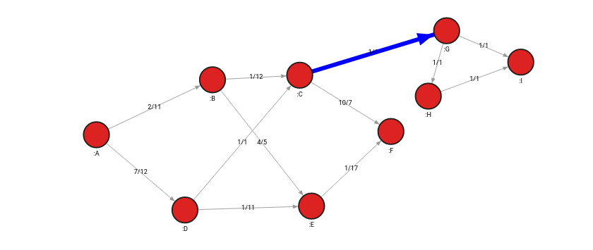
return component_id, count(*);

If nodes C and G become disconnected and the algorithm is rerun, the result will increase to 2 to indicate there are now two disjoint components since the bridge was removed from the graph.

This is a good example of how graph databases utilize the linear time complexity with respect to the size of the graph with an algorithm, while a relational database might spin in neverending loops to answer a simple question like - is my graph connected?

Algorithms like weakly connected components can also be run in impact analysis using the so-called “what-if scenarios”. Parts of the network are connected and disconnected in order to find out what will happen with the network and whether it will stay stable.

Finding well-connected components

The motivation behind finding out what components in the topology are strongly connected together is to make assumptions and analyze the borders of such components. By directly investigating the cross-component relationships, it can be decided if all components are connected well.

An ideal algorithm for that analysis would be community detection, which groups nodes together and assigns them with a community id. Although the algorithm is mostly used to infer hidden links between nodes of the same community, it can also be used to discover links across communities.

The query below will detect all communities in the graph:

CALL community_detection.get()
YIELD node, community_id
SET node.community_id = community_id;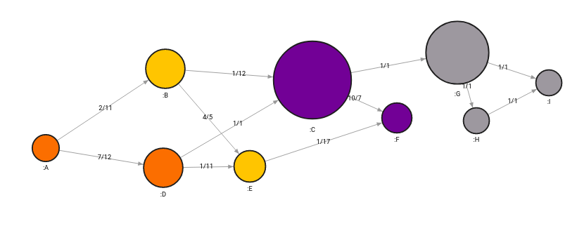

The algorithm detected 4 communities that can be analyzed independently or collapsed together and observed for connections between communities. On a bigger scale, when dealing with the management of oil pipelines across Europe, for example, we can assume that each community represents the network of a specific country and that links between communities could end up being close to borders between countries.

Analyzing separate components of the graph

The whole energy system might be represented with a single dataset, including the entire network topology creating a large graph. However, every data scientist or analyst might be accountable for a different part of the graph, making sure that each subcomponent of the graph (also called subgraph), is well designed and has passed all the criteria. Until now, we have only analyzed graphs as a whole, and algorithms calculated results considering all the nodes and relationships contained in the database.

However, graph projections in Memgraph enable subgraph analysis. The following query will extract a subgraph with the community ID value of 3:

MATCH p=(n)-[r]->(m)
WHERE n.community_id = 3 AND m.community_id = 3
WITH project(p) AS graph
UNWIND graph.nodes + graph.edges AS result
RETURN result;

Every single graph algorithm in Memgraph can be adjusted to work on a subgraph by adding a variable representing a certain path as the first parameter of any algorithm procedure.

Flow analysis

Last but not least, flow analysis is another crucial analysis when dealing with oil and gas pipelines since they can be built differently, have different widths, speeds of flow and the flow at point A might affect the flow at point B. If we look at the network completely, we can therefore calculate the maximum flow that we can pipe through the network, therefore ensuring maximum capacity to the sink nodes which are receiving energy.

To calculate the maximum flow algorithm in Memgraph, use the query below:

MATCH (source:A), (sink:F)
CALL max_flow.get_flow(source, sink, "flow") YIELD max_flow
RETURN max_flow;

If we look at the initial graph, the maximum flow should be 23, with not all the capacity flowing through all the paths, but some paths get partially used since there is an alternative option that, in the end, yields a better flow.

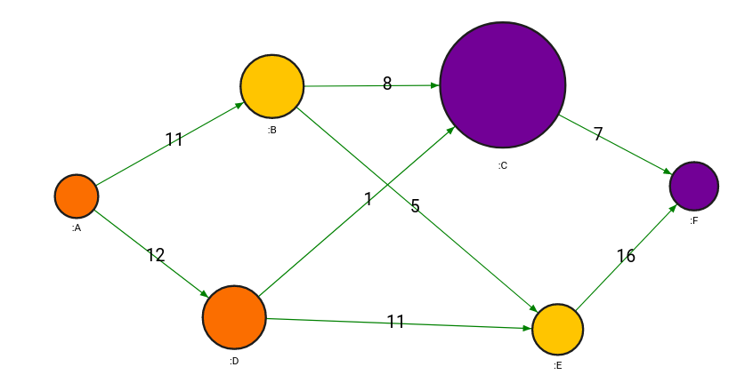
To discover what’s the maximum flow of each relationship, we can use the following query:

MATCH (n)-[r]->(m) SET r.max_flow = 0;

MATCH (source:A), (sink:F)
CALL max_flow.get_paths(source, sink, “flow”) YIELD flow, path
UNWIND relationships(path) AS rel
SET rel.max_flow = flow
RETURN startNode(rel), endNode(rel), rel, flow;

After running the query, we observe the following maximum flow across the network

Conclusion

In this article, we have answered various questions about the network topology, risks and impacts that worry the network systems and managed to get answers quite easily, which would be impossible without the help of a graph database. Except for simple traversals and impact and risk analysis, we also used graph algorithms to do flow analysis, detection of communities and dynamical analysis.

To conclude, graph databases and algorithms are powerful tools that can answer questions regarding energy management topologies and, more importantly, solve any issues with ease and bring immediate insights and value to companies!

For more information about the algorithms Memgraph offers, check out the graph library MAGE and to help you render and visualize data, check out Memgraph Lab.