
Graph Algorithms Cheat Sheet For Coding Interviews
When applying for developer roles, the interviewer might ask you to solve coding problems and some of the most basic ones include graph algorithms like BFS, DFS and Dijkstra's algorithm. You should have a clear understanding of graph algorithms and their data structures if you want to perform well on those challenges. This article will give you an idea of the well-known graph algorithms and data structures to ace your interview. Check out our Graph algorithms infographic for a visual overview of these and other advanced algorithms available in Memgraph.
Let's first cover what a graph data structure is. It is a data structure that stores data in the form of interconnected edges (paths) and vertices (nodes). These data structures have a lot of practical applications. For instance, Facebook's Graph API is a perfect example of the application of graphs to real-life problems. Everything is a vertice or an edge on the Graph API. A vertice is anything that has some characteristic properties and can store data. The vertices of Facebook Graph API are Pages, Places, Users, Events, Comments, etc. On the other hand, every connection is an edge. Examples of Graph API edges are a user posting a comment, photo, video, etc.
Common Operations On Graph Data Structures
A graph data structure (V, E) consists of:
- A collection of nodes or vertices (V)
- A collection of paths or edges (E)
You can manage the graph data structures using the common operations mentioned below.
- contains - It checks if a graph has a certain value.
- addNode - It adds vertices to the graphs.
- removeNode - It removes the vertices from the graphs.
- hasEdge - It checks if a path or a connection exists between any two vertices in a graph.
- addEdge - It adds paths or links between vertices in graphs.
- removeEdge - It removes the paths or connections between vertices in a graph.
Fundamental Graph Algorithms
Let's look at some graph algorithms along with their respective data structures and code examples.
Breadth-First Search (BFS)
It is a graph traversal algorithm that traverses the graph from the nearest node (root node) and explores all unexplored (neighboring) nodes. You can consider any node in the graph as a root node when using BFS for traversal.
You can think of BFS as a recursive algorithm that searches all the vertices of a graph or tree data structure. It puts every vertex of the graph into the following categories.
- Visited
- Non-visited
BFS has a wide variety of applications. For instance, it can create web page indexes in web crawlers. It can also find the neighboring locations from a given source location.
The breadth-first search uses Queue data structure to find the shortest path in a given graph and makes sure that every node is visited not more than once.
Code Example
Below is a Python code example that traverses a graph using the Breadth-first search algorithm.
# Using a BFS algorithm
import collections
def bfs(graph, root):

    visited, queue = set(), collections.deque([root])
    visited.add(root)

    while queue:
        # Dequeuing a vertex from queue
        vertex = queue.popleft()
        print(str(vertex) + " ", end="")

        # If not visited, marking it as visited, and

# enqueuing it
        for neighbor in graph[vertex]:
            if neighbor not in visited:
                visited.add(neighbor)
                queue.append(neighbor)


if __name__ == '__main__':
    graph = {0: [1, 2], 1: [2], 2: [3], 3: [1, 2]}
    print("Below is the Breadth First Traversal: ")
    bfs(graph, 0)
The output is as:

Depth First Search (DFS)
The depth-first search algorithm starts the traversal from the initial node of a given graph and goes deeper until we find the target node or the leaf node (with no children). DFS then backtracks from the leaf node towards the most recent node to explore it.
The Depth-first search algorithm uses Stack data structure. It traverses from an arbitrary node, marks the node, and moves to the adjacent unmarked node.
Code Example
Below is the code example that traverses a graph using the Depth-first search algorithm.
# Using DFS algorithm
def dfs(graph, start, visited=None):
 if visited is None:
        visited = set()
    visited.add(start)

    print(start)

    for next in graph[start] - visited:
        dfs(graph, next, visited)
    return visited


graph = {'0': set(['1', '2']),
         '1': set(['0', '3', '4']),
         '2': set(['0']),
         '3': set(['1']),
         '4': set(['2', '3'])}

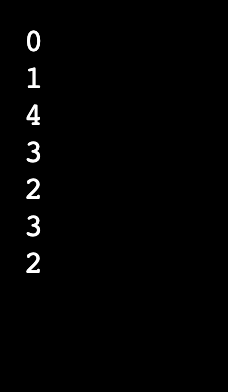
dfs(graph, '0')
The output is as:
Dijkstra Algorithm
Dijkstra algorithm is a shortest path algorithm that computes the shortest path between the source node (given node) and all other neighboring nodes in a given graph. It uses the edges' weights to find a path that minimizes the weight (total distance) between the source node and all other nodes. The most commonly used data structure for the Dijkstra algorithm is Minimum Priority Queue. It is because the operations of this algorithm match with the specialty of a minimum priority queue. The minimum priority queue is a data structure that manages a list of values (keys) and prioritizes the elements with minimum value. It supports the operations like getMin(), extractMin(), insert(element) etc.
Code Example
Below is the code example that computes the shortest distance from every node (source node) to all neighboring nodes using the Dijkstra algorithm.
import sys

# Providing the graph with vertices and edges
v_graph = [[0, 0, 1, 1, 0, 0, 0],
                  [0, 0, 1, 0, 0, 1, 0],
                  [1, 1, 0, 1, 1, 0, 0],
                  [1, 0, 1, 0, 0, 0, 1],
                  [0, 0, 1, 0, 0, 1, 0],
                  [0, 1, 0, 0, 1, 0, 1],
                  [0, 0, 0, 1, 0, 1, 0]]

e_graph = [[0, 0, 1, 2, 0, 0, 0],
               [0, 0, 2, 0, 0, 3, 0],
               [1, 2, 0, 1, 3, 0, 0],
               [2, 0, 1, 0, 0, 0, 1],
               [0, 0, 3, 0, 0, 2, 0],
               [0, 3, 0, 0, 2, 0, 1],
               [0, 0, 0, 1, 0, 1, 0]]

# Finding the vertex that has to be visited next
def node_to_visit():

   global visited_and_distance
    v = -10
    for index in range(vertices):
        if visited_and_distance[index][0] == 0 /
            and (v < 0 or visited_and_distance[index][1] <=
                 visited_and_distance[v][1]):
            v = index
    return v


vertices = len(v_graph[0])

visited_and_distance = [[0, 0]]
for i in range(vertices-1):
    visited_and_distance.append([0, sys.maxsize])

for vertex in range(vertices):

    # Finding next vertex to be visited
    to_visit = node_to_visit()
    for neighbor_index in range(vertices):

        # Updating new distances
        if v_graph[to_visit][neighbor_index] == 1 and /
                visited_and_distance[neighbor_index][0] == 0:
            new_distance = visited_and_distance[to_visit][1] /
                + e_graph[to_visit][neighbor_index]
            if visited_and_distance[neighbor_index][1] > new_distance:
                visited_and_distance[neighbor_index][1] = new_distance

        visited_and_distance[to_visit][0] = 1

i = 0

# Printing the distance
for distance in visited_and_distance:
    print("Computed Distance of ", chr(ord('a') + i),
          " from source vertex is: ", distance[1])
    i = i + 1
The output is as:

Bellman-Ford Algorithm
Like Dijkstra's algorithm, it is also a single-source shortest path algorithm. It computes the shortest distance from a single vertex to all other vertices in a weighted graph. Bellman ford's algorithm guarantees the correct answer even if the weighted graph has negatively weighted edges. However, the Dijkstra algorithm can not guarantee an accurate result in the case of negative edge weights.
Code Example
Below is the code example that computes the shortest distance from a single vertex to other vertices using the Bellman-Ford algorithm.
# Using Bellman-Ford Algorithm
class Graph:

    def __init__(self, vertices):
        self.V = vertices # Vertices in the graph
        self.graph = [] # Array of edges

# Adding edges
    def add_edge(self, s, d, w):
        self.graph.append([s, d, w])

    # Printing the solution
    def print_solution(self, dist):
        print("Vertex Distance from Source")
        for i in range(self.V):
            print("{0}/t/t{1}".format(i, dist[i]))

    def bellman_ford(self, src):

        # Filling the distance array and predecessor array
        dist = [float("Inf")] * self.V
        # Marking the source vertex
        dist[src] = 0

        # Relaxing edges |V| - 1 times
        for _ in range(self.V - 1):
            for s, d, w in self.graph:
                if dist[s] != float("Inf") and dist[s] + w < dist[d]:
                    dist[d] = dist[s] + w

        # Step 3: Detecting negative cycle in a graph
        for s, d, w in self.graph:
            if dist[s] != float("Inf") and dist[s] + w < dist[d]:
                print("Graph contains negative weight cycle")
                return

        # No negative weight cycle found!
        # Printing the distance and predecessor array

        self.print_solution(dist)
g = Graph(5)
g.add_edge(0, 1, 5)
g.add_edge(0, 2, 4)
g.add_edge(1, 3, 3)
g.add_edge(2, 1, 6)
g.add_edge(3, 2, 2)

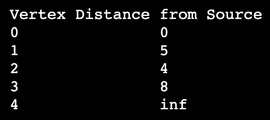
g.bellman_ford(0)
The output is as:
Floyd Warshall Algorithm
The Floyd Warshall algorithm finds the shortest distance between every pair of vertices in a given weighted graph and solves the All Pairs Shortest Path problem. You can use it for both directed and undirected weighted graphs. Weighted graphs are the graphs in which edges have numerical values associated with them. Other names for the Floyd Warshall algorithm are the Roy-Warshall algorithm and the Roy-Floyd algorithm.
Code Example
Below is the code example that finds the shortest distance in a weighted graph using the Floyd Warshall algorithm.
# Total number of vertices
vertices = 4

INF = 999

# implementing the floyd-warshall algorithm
def floyd_warshall(Graph):
    distance = list(map(lambda a: list(map(lambda b: b, a)), Graph))

    # Adding the vertices individually
    for k in range(vertices):
        for a in range(vertices):
            for b in range(vertices):
                distance[a][b] = min(distance[a][b], distance[a][k] + distance[k][b])
    solution(distance)


# Printing the desired solution
def solution(distance):
    for a in range(vertices):
        for b in range(vertices):
            if(distance[a][b] == INF):
                print("INF", end=" ")
            else:
                print(distance[a][b], end=" ")
        print(" ")


Graph = [[0, 3, INF, 5],
         [2, 0, INF, 4],
         [INF, 1, 0, INF],
         [INF, INF, 2, 0]]
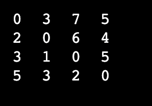
floyd_warshall(Graph)
The output is as:
Prim's Algorithm
It is a greedy algorithm that finds the minimum spanning tree for a weighted undirected graph. Let's look at the main terms associated with this algorithm.
- Spanning Tree - It is the subgraph of an undirected connected graph.
- Minimum Spanning Tree - It is the spanning tree with the minimum sum of the weights of the edges.
Prim's algorithm traverses the adjacent nodes with all connecting edges at every step. It has many applications such as:
- Making network cycles
- Laying down electrical wiring cables
- Network designing
Code Example
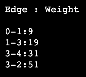
Below is the code example that finds all edges with their respective weights using Prim's algorithm.
INF = 9999999
# graph's vertices
vertices = 5

# graph representation
graph = [[0, 9, 75, 0, 0],
         [9, 0, 95, 19, 42],
         [75, 95, 0, 51, 66],
         [0, 19, 51, 0, 31],
         [0, 42, 66, 31, 0]]

# creating an array for tracking the selected vertex
selected_vertex = [0, 0, 0, 0, 0]
# setting the number of edges to 0
number_of_edges = 0

# choosing 0th vertex and setting it to True
selected_vertex[0] = True
# printing the edge and the corresponding weight
print("Edge : Weight/n")
while (number_of_edges < vertices - 1):
    min = INF
    a = 0
    b = 0
    for i in range(vertices):
        if selected_vertex[i]:
            for j in range(vertices):
                if ((not selected_vertex[j]) and graph[i][j]):
                    if min > graph[i][j]:
                        min = graph[i][j]
                        a = i
                        b = j
    print(str(a) + "-" + str(b) + ":" + str(graph[a][b]))
    selected_vertex[b] = True
    number_of_edges += 1
The output is as:
Kruskal's Algorithm
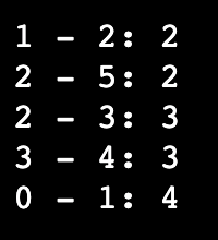
It finds the minimum spanning tree for a connected weighted graph. Its main objective is to find the subset of the edges through which we can traverse every graph's vertex. This algorithm uses the greedy approach to find the optimum solution at every stage rather than focusing on a global optimum.
Kruskal's algorithm starts from the edges having the lowest weights and keeps adding the edges until you achieve the goal. Below are the steps to implement this algorithm.
- Sort all edges in the ascending order of weight (low to high).
- Take the lowest weight edge and add it to the spanning tree. Reject the edge that creates a cycle when added.
- Keep adding the edges until we cover all vertices and make a minimum spanning tree.
Code Example
Below is the code example that finds a subset of edges and computes a minimum spanning tree using Kruskal's algorithm.
class Graph:
    def __init__(self, vertices):
        self.V = vertices
        self.graph = []

    def add_edge(self, u, v, w):
        self.graph.append([u, v, w])

    # Search function

    def find(self, parent, i):
        if parent[i] == i:
            return i
        return self.find(parent, parent[i])

def apply_union(self, parent, rank, x, y):
        xroot = self.find(parent, x)
        yroot = self.find(parent, y)
        if rank[xroot] < rank[yroot]:
            parent[xroot] = yroot
        elif rank[xroot] > rank[yroot]:
            parent[yroot] = xroot
        else:
            parent[yroot] = xroot
            rank[xroot] += 1

    # Applying Kruskal’s algorithm
    def kruskal_algo(self):
        result = []
        i, e = 0, 0
        self.graph = sorted(self.graph, key=lambda item: item[2])
        parent = []
        rank = []
        for node in range(self.V):
            parent.append(node)
            rank.append(0)
        while e < self.V - 1:
            u, v, w = self.graph[i]
            i = i + 1
            x = self.find(parent, u)
            y = self.find(parent, v)
            if x != y:
                e = e + 1
                result.append([u, v, w])
                self.apply_union(parent, rank, x, y)
        for u, v, weight in result:
            print("%d - %d: %d" % (u, v, weight))

g = Graph(6)
g.add_edge(0, 1, 4)
g.add_edge(0, 2, 4)
g.add_edge(1, 2, 2)
g.add_edge(1, 0, 4)
g.add_edge(2, 0, 4)
g.add_edge(2, 1, 2)
g.add_edge(2, 3, 3)
g.add_edge(2, 5, 2)
g.add_edge(2, 4, 4)
g.add_edge(3, 2, 3)
g.add_edge(3, 4, 3)
g.add_edge(4, 2, 4)
g.add_edge(4, 3, 3)
g.add_edge(5, 2, 2)
g.add_edge(5, 4, 3)
g.kruskal_algo()
The output is as:
Topological Sort Algorithm
It is a linear ordering of the vertices of a directed acyclic graph (DAG) in which vertex x occurs before vertex y when ordering the directed edge xy from vertex x to vertex y. For instance, the graph's vertices can represent jobs to be completed, and the edges can depict the requirements that one task must be completed before another.
Code Example
Below is the code example that linearly orders the vertices using the Topological Sort algorithm.
from collections import defaultdict

# making a Class for representing a graph
class Graph:
	def __init__(self, vertices):
    	# dictionary that contains adjacency List
		self.graph = defaultdict(list)
        # number of vertices
		self.V = vertices

	# function for adding an edge to graph
	def addEdge(self, u, v):
		self.graph[u].append(v)

	# A recursive function used by topologicalSort
	def topologicalSortUtil(self, v, visited, stack):

		# Marking the current node as visited.
		visited[v] = True


		for i in self.graph[v]:
			if visited[i] == False:
				self.topologicalSortUtil(i, visited, stack)

		# Pushing current vertex to stack that stores result
		stack.append(v)

	# Topological Sort function.
	def topologicalSort(self):

		# Marking all the vertices as not visited
		visited = [False]*self.V
		stack = []


		# the sort starts from all vertices one by one
		for i in range(self.V):
			if visited[i] == False:
				self.topologicalSortUtil(i, visited, stack)

		# Printing contents of the stack
		print(stack[::-1])
g = Graph(6)
g.addEdge(5, 2)
g.addEdge(5, 0)
g.addEdge(4, 0)
g.addEdge(4, 1)
g.addEdge(2, 3)
g.addEdge(3, 1)

print ("The topological sort of the given graph is as")


g.topologicalSort()
The output is as:

Johnson's Algorithm
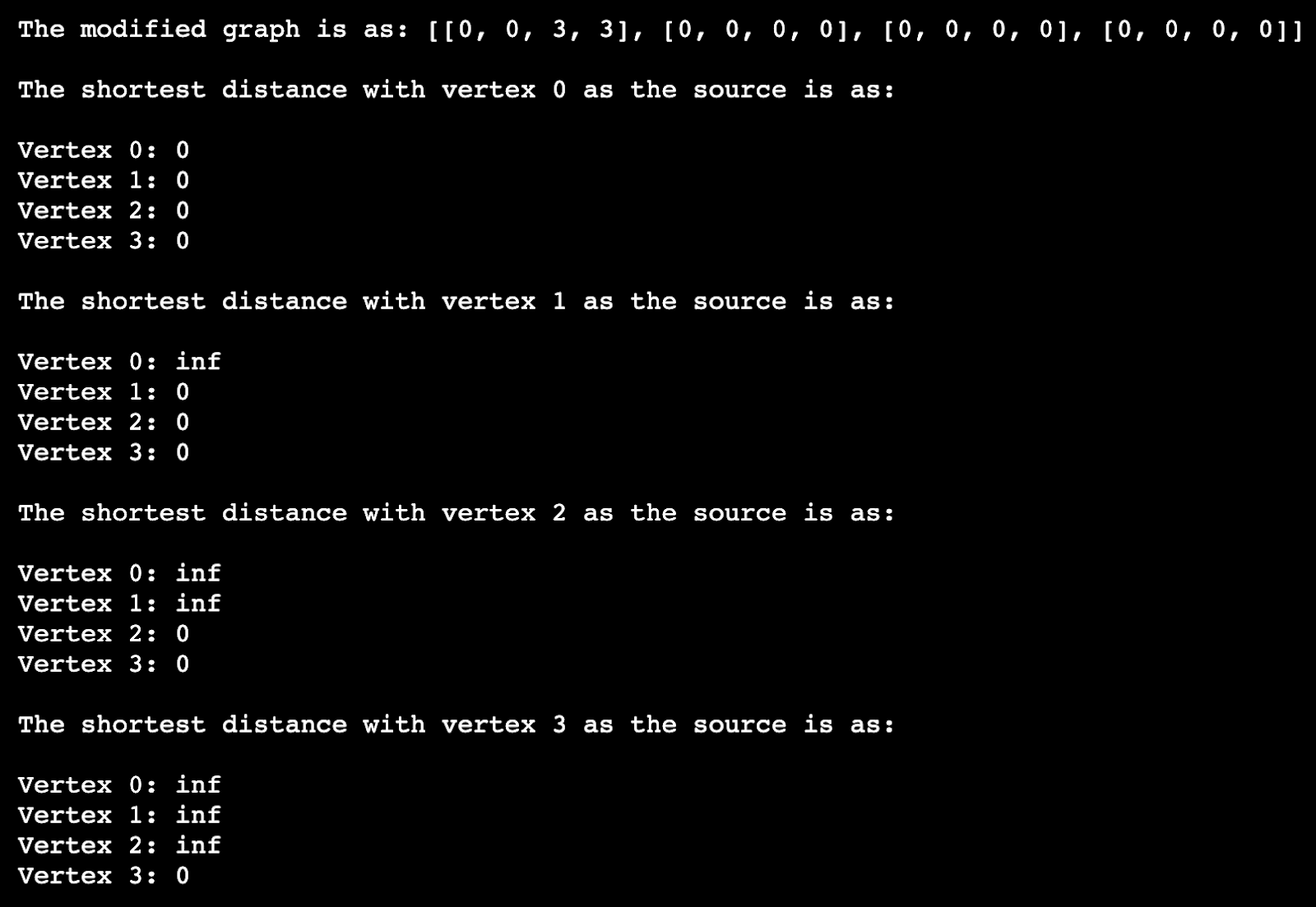
Johnson's algorithm finds the shortest path between every pair of vertices in a given weighted graph where weights can also be negative. It uses the technique of reweighting.
If a given graph has non-negative edge weights, we find the shortest path between all pairs of vertices by running Dijkstra's algorithm. However, if a graph contains negatively weighted edges, we calculate a new set of non-negative weighted edges and use the same method.
Code Example
Below is the code example that computes the shortest distance by sorting vertices using Johnson’s algorithm.
from collections import defaultdict
MAX_INT = float('Inf')
# the function returns the vertex with minimum weight
def min_distance(dist, visited):

    (min, min_vertex) = (MAX_INT, 0)
    for v in range(len(dist)):
        if min > dist[v] and visited[v] == False:
            (min, min_vertex) = (dist[v], v)

    return min_vertex


# removing negative weights
def Dijkstra_algo(graph, modified_graph, src):

    # vertices in the graph
    vertices = len(graph)

    # Dictionary for checking if a given vertex is
    # in the shortest path tree
    sptSet = defaultdict(lambda : False)

    # computing distance of all vertices from the source

    for count in range(vertices):

        # The current vertex that is not yet included in the
        # shortest path tree
        currentV = min_distance(distance, sptSet)
        sptSet[currentV] = True

        for v in range(vertices):
            if ((sptSet[v] == False) and
                (distance[v] > (distance[currentV] +
                modified_graph[currentV][v])) and
                (graph[currentV][v] != 0)):

                distance[v] = (distance[currentV] +
                                modified_graph[currentV][v]);

    # Printing the Shortest distance from the source
    for v in range(vertices):
        print ('Vertex ' + str(v) + ': ' + str(distance[v]))

# computing shortest distances
def Bellman_algo(edges, graph, vertices):

    # Adding a source and calculating its min
    # distance from other nodes
    distance = [MAX_INT] * (vertices + 1)
    distance[vertices] = 0

    for a in range(vertices):
        edges.append([vertices, a, 0])

    for a in range(vertices):
        for (src, des, weight) in edges:
            if((distance[src] != MAX_INT) and
                    (distance[src] + weight < distance[des])):
                distance[des] = distance[src] + weight


    return distance[0:vertices]

# Function for implementing Johnson Algorithm
def Johnson_algo(graph):

    edges = []

    # Creating a list of edges for Bellman-Ford Algorithm
    for a in range(len(graph)):
        for b in range(len(graph[a])):

            if graph[a][b] != 0:
                edges.append([a, b, graph[a][b]])

    # Weights for modifying the original weights
    modify_weights = Bellman_algo(edges, graph, len(graph))

    modified_graph = [[0 for x in range(len(graph))] for y in
                    range(len(graph))]

    # Modifying the weights to get rid of negative weights
    for a in range(len(graph)):

        for b in range(len(graph[a])):

            if graph[a][b] != 0:
                modified_graph[a][b] = (graph[a][b] +
                        modify_weights[a] - modify_weights[b]);

    print ('The modified graph is as: ' + str(modified_graph))

    # Running Dijkstra for every vertex
    for src in range(len(graph)):
        print ('/nThe shortest distance with vertex ' +
                        str(src) + ' as the source is as:/n')
        Dijkstra_algo(graph, modified_graph, src)


graph = [[0, -5, 2, 3],
         [0, 0, 4, 0],
         [0, 0, 0, 1],
         [0, 0, 0, 0]]

Johnson_algo(graph)
The output is as:
Kosaraju's Algorithm
It is a depth-first search-based algorithm that finds the strongly connected components in a graph. Kosaraju's algorithm is based on the concept that if one can reach a vertex y starting from vertex x, one should reach vertex x starting from vertex y. If it is the case, we can say that the vertices x and y are strongly connected.
Code Example
Below is the code example that determines whether the graph is strongly connected using Kosaraju’s algorithm.
# Using Kosaraju's algorithm to check if a given directed graph is
# strongly connected or not

from collections import defaultdict

class Graph:

	def __init__(self, vertices):
     	# vertices of a graph
		self.V = vertices
        # dictionary for storing a graph
		self.graph = defaultdict(list)

	# function for adding an edge to graph
	def addEdge(self, u, v):
		self.graph[u].append(v)

	# A function for performing DFS
	def DFSUtil(self, v, visited):

		# Marking the current node as visited
		visited[v] = True


		for i in self.graph[v]:
			if visited[i] == False:
				self.DFSUtil(i, visited)

	# Function returning the transpose of this graph

	def getTranspose(self):

		g = Graph(self.V)


		for i in self.graph:

			for j in self.graph[i]:
				g.addEdge(j, i)

		return g

	# main function returns true if the graph is strongly connected
	def isSC(self):

		# Marking all the vertices as not visited for 1st DFS
		visited =[False]*(self.V)

		# Performing DFS traversal starting from the first vertex.
		self.DFSUtil(0,visited)

		# Return false if DFS traversal doesn't visit all vertices
		if any(i == False for i in visited):
			return False

		# Creating a reversed graph
		gr = self.getTranspose()

		# Marking all the vertices as not visited for 2nd DFS
		visited =[False]*(self.V)

		# Doing DFS for the reversed graph starting from the first vertex.
		# Starting Vertex must be same starting point of first DFS
		gr.DFSUtil(0,visited)

		# returning false if all vertices are not visited in second DFS
		if any(i == False for i in visited):
			return False

return True

# Considering a random graph
g1 = Graph(5)
g1.addEdge(0, 1)
g1.addEdge(1, 2)
g1.addEdge(2, 3)
g1.addEdge(3, 0)
g1.addEdge(2, 4)
g1.addEdge(4, 2)
print ("Yes the graph is strongly connected." if g1.isSC() else "Not strongly connected")

g2 = Graph(4)
g2.addEdge(0, 1)
g2.addEdge(1, 2)
g2.addEdge(2, 3)
print ("Yes the graph is strongly connected." if g2.isSC() else "Not strongly connected")
The output is as:

Conclusion
So far, we discussed that graphs are non-linear data structures that consist of nodes and edges. We can use graphs to solve many real-life problems. For instance, they are used in social networking sites like Facebook, Linkedin, etc. Each person can be denoted with a vertex on Facebook. Likewise, each node can contain information like name, gender, personID, etc. Further, we discussed some well-known graph algorithms like:
- Breadth-First Search - Computes the shortest path in a given graph using a Queue data structure.
- Depth-First Search - Uses a Stack data structure to find the shortest path in a given graph.
- Dijkstra Algorithm - Uses a Minimum priority queue data structure to find the shortest path between the source node and other given nodes in a graph.
- Bellman-Ford Algorithm - Single source shortest path algorithm like Dijkstra's algorithm.
- Floyd Warshall Algorithm - Solves the All Pairs shortest path problem.
- Prim's Algorithm - It finds the minimum spanning tree for an undirected weighted graph.
- Kruskal's Algorithm - It finds the minimum spanning tree for a connected weighted graph.
- Topological Sort Algorithm - Represents a linear ordering of vertices in a directed acyclic graph.
- Johnson's Algorithm - Finds the shortest path between every pair of vertices where weights can also be negative.
- Kosaraju's Algorithm - Finds the strongly connected components in a graph.
If you need more info or help with understanding a graph algorithm, join the Memgraph Discord server and ask away.