How to Build a Route Planning Application with Breadth First Search and Dijkstra's Algorithm

By Karim Traiaia

12 min readJune 9, 2020

Introduction

One of the most common applications of graph traversal algorithms is route planning and optimization problems. These can vary from simple things like finding the shortest path from a starting point to a destination to more complex scenarios where it is required to pass a particular intermediate node (e.g. A specific city) and satisfy multiple conditions (e.g. Limited number of stops) before reaching the final destination. Some practical examples include:

Logistics and supply chain optimization – Planning effective routes to minimize cost, increase vehicle utilization and improve operations by taking into account things like travel distance, vehicle capacity, road tolls, fuel consumption, and border taxes.
Travel route planning – Finding the quickest way to get from point A to point B taking into account things like traffic, road closures, and construction.
Network optimization – Improving communications and information transfer in telephone and cellular networks by finding optimal paths based on factors such as bandwidth.

In this tutorial, we will build a simple graph application with Memgraph and Cypher to navigate the European road network and learn how to use some of the most popular graph algorithms used to solve routing problems including breadth-first search (BFS), and Dijkstra's algorithm.

Prerequisites

To follow along, you will need the following:

A local installation of Memgraph. You can refer to the Memgraph documentation.
A local installation of Memgraph Lab.
Basic knowledge of the Cypher query language.
[OPTIONAL] If you don't want to install Memgraph & Memgraph Lab on your own you can create a free account on Memgraph Cloud

Step 1 — Defining The Data Model

In this step, you will define your data model as a connected graph of nodes (Vertices) and relationships (Edges) along with their properties and labels.

For this tutorial, you will be using the European road network which consists of 999 major cities and 39 countries. The data model, in this case, is quite simple.

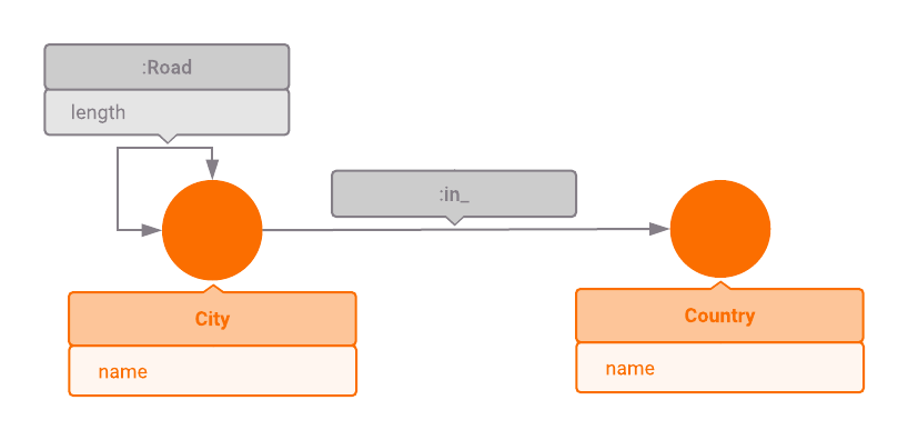
The graph contains two node types and two relationship types. Every city is connected to the country it belongs to via a relationship of type(Lable) :In_ and to other cities less than 500 kilometers via a relationship of type :Road. The Distance between cities is specified in the length property of the relationship.

Now that you have defined the data model, you're ready to import the dataset.

Step 2 — Importing Data Into Memgraph Using Cypher

The easiest way to import our dataset into Memgraph is using Cypher queries.

You can download the dataset file containing Cypher queries from here. If you unzip the file, you will get the file with a .cypherl extension. You can load it to Memgraph via Memgraph LAB.
Memgraph LAB has an import/export tab for importing the .cypherl files. If you need help importing it, you can follow docs for importing Cypher queries

If you open the .cyhperl file in any text or code editor, you will notice that the first few Cypher statements are for creating indexes and the rest of the statements for loading data. If you didn't have a file to import the data, you would manually crate index and import the data by executing queries. If you want to find out how to do it, follow the manual import section or feel free to skip it.

Manual import

You can import the data by manually executing queries like this:

CREATE (:Country {name: "Croatia"});

If you want to create an index on the name property of country nodes to improve search performance when looking for specific countries, you can do it with Memgraph!

[NOTE] A database index essentially creates a redundant copy of some of the data in the database to improve the efficiency of searches for the indexed data. However, this comes at the cost of additional storage space and more writing, so deciding what to index and not to the index is important.

To create an index, we can use the following Cypher query:

CREATE INDEX ON :Country(name);

Now that we have created the country nodes, we are ready to add the cities associated with each country. To do this, you can execute the following query:

MATCH (country:Country {name: "Croatia"}) CREATE (city:City {name: "Osijek"})-[:In_]->(country);

Next, we create an index on the name property of City nodes:

CREATE INDEX ON :City(name);

Now that we have created all the nodes in our graph, we will create the relationships between them. As described in our data model, there are two types of relationships. A relationship of type(Lable) :In_, and a relationship of type :Road which contains a property of type Length. To create the relationships you can execute the following query:

MATCH (city1:City {name: "Banja Luka"})-[:In_]->(:Country {name: "Bosnia and Herzegovina"})
MATCH (city2:City {name: "Osijek"})-[:In_]->(:Country {name: "Croatia"})
CREATE (city1)-[:Road {length: 214.51}]->(city2);

You now have the dataset loaded inside Memgraph and ready to be queried. In the next step, you will run a few basic queries to learn how to use the breadth-first search and Dijkstra’s algorithm for finding the shortest paths between nodes in the graph.

Step 3 — Using the Breadth-First Search Algorithm to Find and Filter Paths

To get started, let's make sure that the data has been correctly imported into Memgraph by running the following simple Cypher query to return all the countries found in the database:

MATCH (c:Country) RETURN c.name;

This query matches and returns all nodes with label Country. If everything works properly, you should get a list of 39 countries.

Now let’s explore a few pathfinding queries to demonstrate the power of graph databases. After all, this is what really sets graph databases apart from SQL and other NoSQL systems.

Say you want to drive from Paris to Berlin and want to plan your route to minimize the number of stops. You also don't want to drive more than 500 Km between stops. Since the edges in our road network don't connect cities that are more than 500 km apart, this is a great use case for the breadth-first search (BFS) algorithm.

Although Cypher, as defined through the openCypher project, doesn't offer a feature for BFS, Memgraph provides a custom implementation.

To execute a breadth-first search (BFS) algorithm, we will run the following query:

MATCH p = (:City {name: "Paris"}) -[:Road * bfs]->(:City {name:"Berlin"}) RETURN nodes(p);

This query will return the nodes along a path p with the smallest number of hopes starting from the city Paris and connecting it to the cityBerlin through the relationship of type or lableRoad. You should get the following result:

+------------------------------------------------------------------------------------------------------------+
| nodes (p)
+------------------------------------------------------------------------------------------------------------+
| [(:City {name: "Paris"}), (:City {name: "Düsseldorf"}), (:City {name: "Kiel"}), (:City {name: "Berlin"})] |
+------------------------------------------------------------------------------------------------------------+

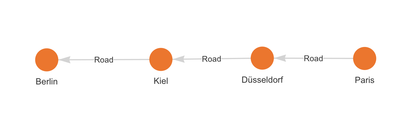
If you're working with Memgraph Lab and would like to visualize the path, you would modify the query to return p instead of nodes(p). This will return both nodes and relationships along the shortest path between Paris and Berlin. The query should be:

MATCH p = (:City {name: "Paris"}) -[:Road * bfs]->(:City {name:"Berlin"}) RETURN p;

The output should be:

Now, let’s suppose that instead of driving to Berlin, you decided to go on a biking road trip with your friends. As a result, you want to limit yourself to cities that are no more than 200 Km apart since that’s the maximum you want to bike per day. To do this, you can run the following query:

MATCH p = (:City {name: "Paris"})
          -[:Road * bfs (e, v | e.length <= 200)]->
          (:City {name: "Berlin"})
RETURN nodes(p);

The output should be:

+-----------------------------------------------------------------------------------------------------------------------------------------------------------------------------------------------------------------+
| nodes(p)                                                                                                                                                                                                        |
+-----------------------------------------------------------------------------------------------------------------------------------------------------------------------------------------------------------------+
| [(:City {name: "Paris"}), (:City {name: "Reims"}), (:City {name: "Metz"}), (:City {name: "Worms"}), (:City {name: "Würzburg"}), (:City {name: "Erfurt"}), (:City {name: "Leipzig"}), (:City {name: "Berlin"})] |
+-----------------------------------------------------------------------------------------------------------------------------------------------------------------------------------------------------------------+

As you can see, we added a special syntax to the query (e, v | e.length <= 200). This is called a filter lambda. It's a function that takes an edge symbol e and a vertex symbol v and decides whether this edge and vertex pair should be considered valid in breadth-first expansion by returning true or false (or Null). In the above example, lambda is returning true if the edge length is not greater than 200, due to the fact that we don't want to bike more than 200 km in one go.

The filter lambda function can also be extended to support several other constraints. As an example, let's say you don't want to visit the city of Metz. In this case, you will run the following query:

MATCH p = (:City {name: "Paris"})
          -[:Road * bfs (e, v | e.length <= 200 AND v.name != "Metz")]->
          (:City {name: "Berlin"})
RETURN nodes(p);

Now you can see that your result has changed and the new cities you'll be visiting on your trip are:

+---------------------------------------------------------------------------------------------------------------------------------------------------------------------------------------------------------------------------------+
| nodes(p)                                                                                                                                                                                                                        |
+---------------------------------------------------------------------------------------------------------------------------------------------------------------------------------------------------------------------------------+
| [(:City {name: "Paris"}), (:City {name: "Reims"}), (:City {name: "Charleroi"}), (:City {name: "Venlo"}), (:City {name: "Gütersloh"}), (:City {name: "Göttingen"}), (:City {name: "Halle (Saale)"}), (:City {name: "Berlin"})] |
+---------------------------------------------------------------------------------------------------------------------------------------------------------------------------------------------------------------------------------+

Step 4 — Using Dijkstra's Algorithm to Find the Shortest Path

So far you were planning your trip based by taking into consideration the number of stops you’ll be making, but what if you wanted to find the quickest route or shortest path between Paris and Berlin based on distance? This is where Dijkstra’s algorithm comes in handy. Let’s find out the shortest path between Paris and Berlin and the cities you’ll be stopping at along the way.

To do this, we will run the following Cypher query:

MATCH p = (:City {name: "Paris"})
          -[:Road * wShortest (e, v | e.length) total_weight]->
          (:City {name: "Berlin"})
RETURN nodes(p) as cities, total_weight;

The output should be:

+------------------------------------------------------------------------------------------------------------+---------------+
| cities                                                                                                     | total_weight  |
+------------------------------------------------------------------------------------------------------------+---------------+
| [(:City {name: "Paris"}), (:City {name: "Heerlen"}), (:City {name: "Hannover"}), (:City {name: "Berlin"})] | 1055.63       |
+------------------------------------------------------------------------------------------------------------+---------------+

As you can see, the syntax is quite similar to breadth-first search syntax. Instead of a filter lambda, we need to provide a weight lambda and the total weight symbol. Given an edge and vertex pair, the weight lambda must return the cost of expanding to the given vertex using the given edge. The path returned will have the smallest possible sum of costs and it will be stored in the total weight symbol. A limitation of Dijkstra's algorithm is that the cost can't be negative.

Let’s now assume you want to find the quickest route for your biking road trip where you don’t want to travel more than 200 km between stops. Just like you did for the breadth-first search query, you can add filters to the lambda function. In this case, you will need to specify that the length for every road e.length must be smaller than 200 km.

To get your result, you'll run the following query:

MATCH p = (:City {name: "Paris"})
      -[:Road * wShortest (e, v | e.length) total_weight (e, v | e.length <= 200)]->
      (:City {name: "Berlin"})
RETURN nodes(p) as cities, total_weight;

Your result should be:

+-----------------------------------------------------------------------------------------------------------------------------------------------------------------------------------------------------------------------+--------------+
| cities                                                                                                                                                                                                                | total_weight |
+-----------------------------------------------------------------------------------------------------------------------------------------------------------------------------------------------------------------------+--------------+
| [(:City {name: "Paris"}), (:City {name: "Reims"}), (:City {name: "Charleroi"}), (:City {name: "Heerlen"}), (:City {name: "Hamm"}), (:City {name: "Hannover"}), (:City {name: "Magdeburg"}), (:City {name: "Berlin"})] | 1105.72      |
+-----------------------------------------------------------------------------------------------------------------------------------------------------------------------------------------------------------------------+--------------+

Conclusion

Congratulations! You just built a simple route planning application by leveraging Memgraph and Cypher. Along the way, you learned how to use the breadth-first search algorithm and Dijkstra’s algorithm to navigate a complex network of inter-connected data using Cypher queries and filtered your results using the powerful and flexible lambda function.