Riding the Berlin subway: a Graph Database Adventure with Memgraph Lab

November 7, 2023

Kruno Golubic

Just as the labyrinth of train tracks intricately connects the bustling stations across geographic areas, forming a network of pathways and possibilities, relationships in graph databases serve to connect nodes in a complex yet orderly web of data. Each station within this network can boast multiple connections, mirroring the multifaceted relationships that can exist between nodes in a graph database.

Think of it this way: each connection between stations is unique, characterized by various properties such as the subway lines that traverse it, the distance it covers, and the number of passengers it ferries daily. These connections are not just lines on a map; they are vital arteries that keep the city alive and moving. Similarly, in the world of graph databases, the relationships between nodes are enriched with properties that add depth, context, and meaning to the network.

The Berlin subway system, with its complexity and efficiency, serves as a captivating analogy and an ideal introduction to the world of graphs. It is a tangible example of how connections and relationships form the backbone of transportation networks and graph databases. In this blog post, we will explore the Berlin subway system using Memgraph Lab. Together, we will uncover the secrets hidden within the data, learn how to visualize complex relationships and gain insights that can only be derived from a graph-centric point of view.

Getting the data on the Berlin subway

Before we can start exploring, we need to get our hands on the data. While I was looking for data on the Berlin subway I came across different datasets related to Berlin subway. I really liked the GitHub gist by Clifford Anderson on Berlin subway, OpenStreetMap data, individual pages about each subway station and line on Wikipedia and I’ve also done some chatting with ChatGPT. With so much available data, first, I needed to decide what I wanted to do with data, and which data I needed to prepare. I decided to start on the small scale. I’ve gathered the data on subway stations and lines that are connecting them in CSV files.

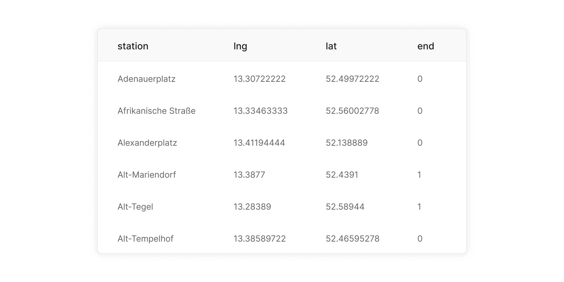
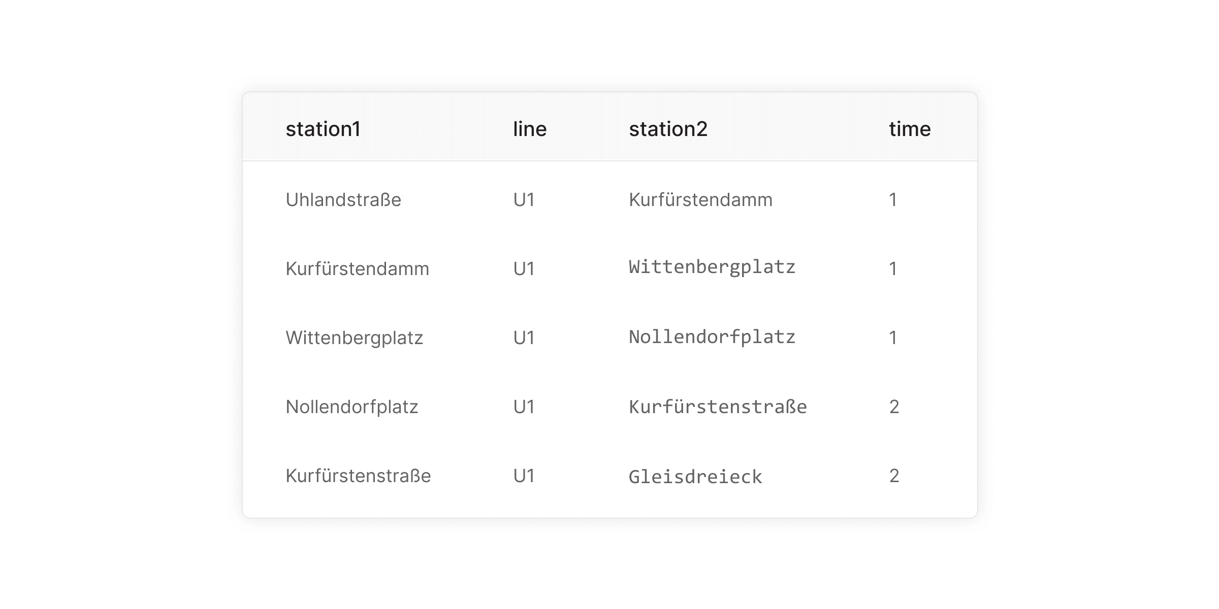
The berlin-stations.csv file contains information about each subway station, including its name, latitude, longitude, and a flag indicating if it’s an end station. The berlin-lines.csv file describes the connections between stations, the subway line they belong to, and the travel time.

I’ve used lng and lat as the names for the columns that hold geographical longitude and latitude to ensure that the stations will be visualized on the map.

berlin stations sample

berlin stations sample 2

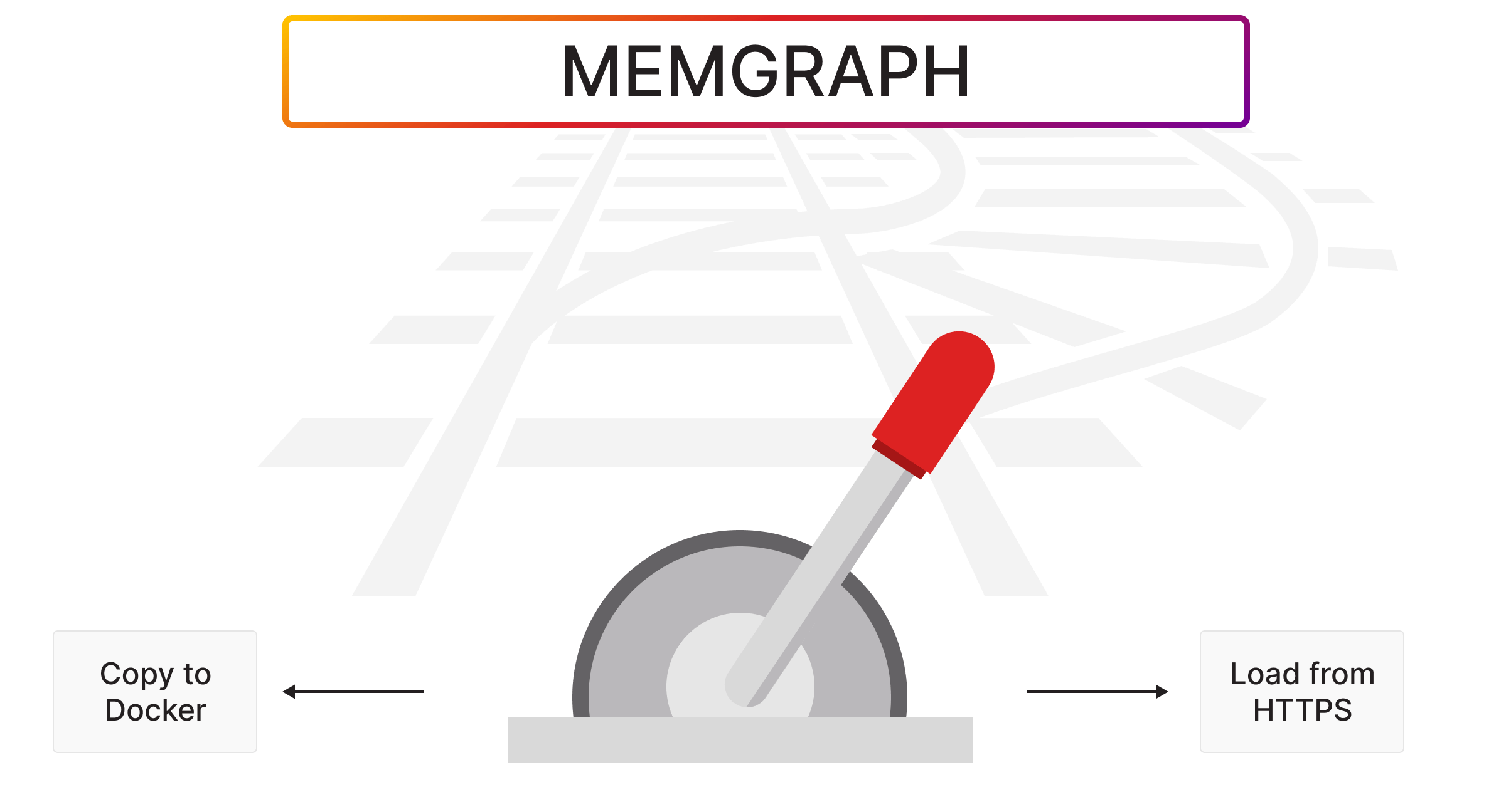
Now that the data is in order, it is time to get it into Memgraph. To get the data about nodes (subway stations) and relationships (subway lines) from the CSV files into Memgraph, use the LOAD CSV Cypher clause. You can either download the CSV files that we’ve prepared for you, or you can import them directly from our website:

It doesn't matter which line you choose, you will end up at the same destination - Memgraph instance loaded with Berlin subway data.

copy to docker

Importing the data on the Berlin subway

I’ve opted to use Docker image with Memgraph Platform for this blog post because Memgraph Platform has everything that I need: the database, algorithms, and a visualization tool. You can also use Memgraph Cloud. In that case, you can only import data by using the URL of the CSV file. If you decide to use the Docker image, both methods mentioned below are valid. :)

If this is the first time that you are hearing about Docker, check out the first steps with Docker on Memgraph's documentation page. Once you have installed Docker, it is time to pull the latest version of Memgraph Platform into the Docker:

docker run -ti -p 3000:3000 -p 7687:7687 -p 7444:7444 --name berlin-subway memgraph/memgraph-platform:latest

With this command, you will create a Docker container named berlin-subway. This will make it easier for you to copy files to your container, or to stop and start the Docker container. Maybe it is not the right time to talk about stopping and staring containers, but since I’ve touched on that topic, here is how it is done. To stop a container, run the following command docker stop berlin-subway in the terminal, and to spin it back up, run docker start berlin-subway. Stopping and starting the containers using these commands ensures that you always spin the container with the Berlin data in it, instead of creating a new empty container.

Import data into Memgraph

To load the data directly from Memgraph’s website, you can use the LOAD CSV command with the appropriate URL. The query looks like this:

LOAD CSV FROM "https://public-assets.memgraph.com/berlin-subway/berlin-stations.csv" WITH HEADER AS row
CREATE (n:Station {name: row.station, lat: toFloat(row.lat), lng: toFloat(row.lng), end: toInteger(row.end )});

LOAD CSV FROM "https://public-assets.memgraph.com/berlin-subway/berlin-lines.csv" WITH HEADER AS row
MATCH (s1:Station {name: row.station1}), (s2:Station {name: row.station2})
CREATE (s1)-[:CONNECTED_VIA {line: row.line, time: ToInteger(row.time)}]->(s2);

If you don’t have Internet connection from your Docker container, you can download the CSV files containing the subway station and line information. Once you download them on your local machine, use the following Docker commands to copy them into the appropriate directory in your Memgraph container:

docker cp berlin-stations.csv berlin-suwbay:/usr/lib/memgraph/berlin-stations.csv

docker cp berlin-lines.csv berlin-subway:/usr/lib/memgraph/berlin-lines.csv

Now open up Memgraph Lab using https://localhost:3000, and run the following Cypher query to get the data into Memgraph:

LOAD CSV FROM "/usr/lib/memgraph/berlin-stations.csv" WITH HEADER AS row
CREATE (n:Station {name: row.station, lat: toFloat(row.lat), lng: toFloat(row.lng), end: toInteger(row.end )});

LOAD CSV FROM "/usr/lib/memgraph/berlin-lines.csv" WITH HEADER AS row
MATCH (s1:Station {name: row.station1}), (s2:Station {name: row.station2})
CREATE (s1)-[:CONNECTED_VIA {line: row.line, time: ToInteger(row.time)}]->(s2);

Visualize data in Memgraph Lab

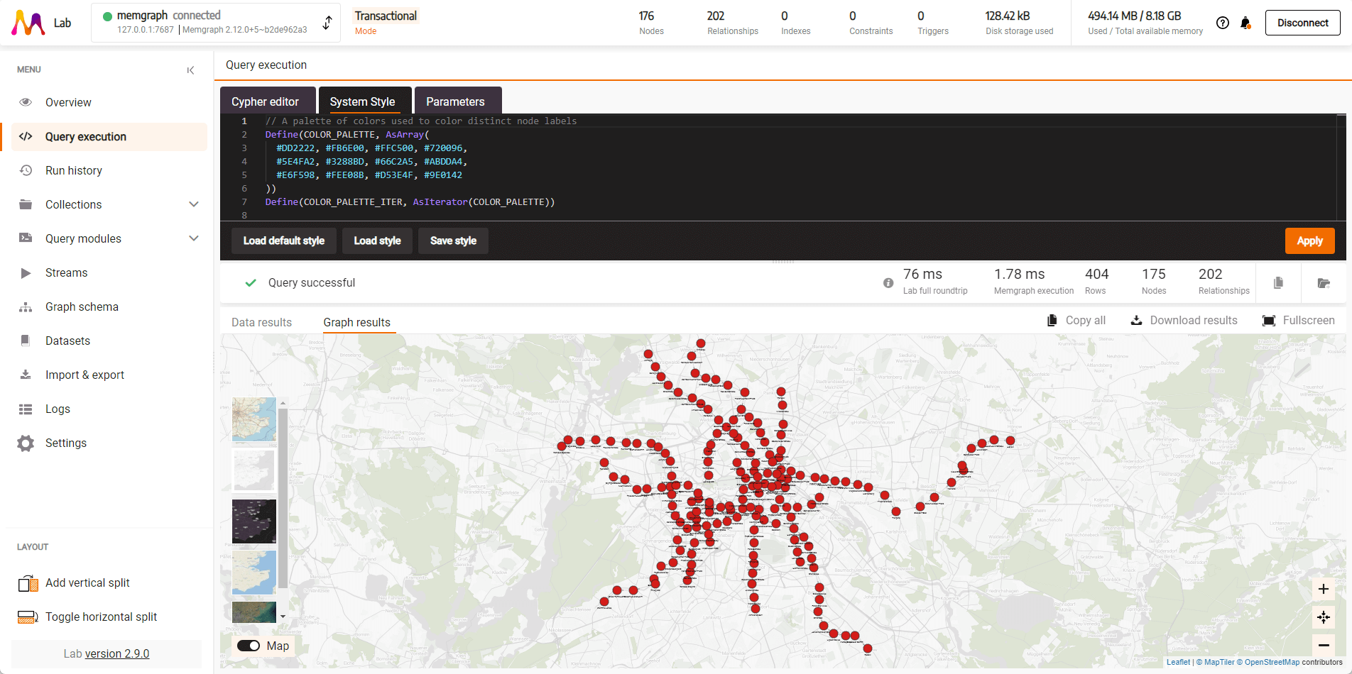
With the data successfully imported, let’s move on to the exciting part - visualization! Let’s start with an easy one. To see all of the stations (nodes) and lines (relations) run this query:

MATCH (n)-[r]-(m)
RETURN n, r, m;

You should get a result similar to this one.

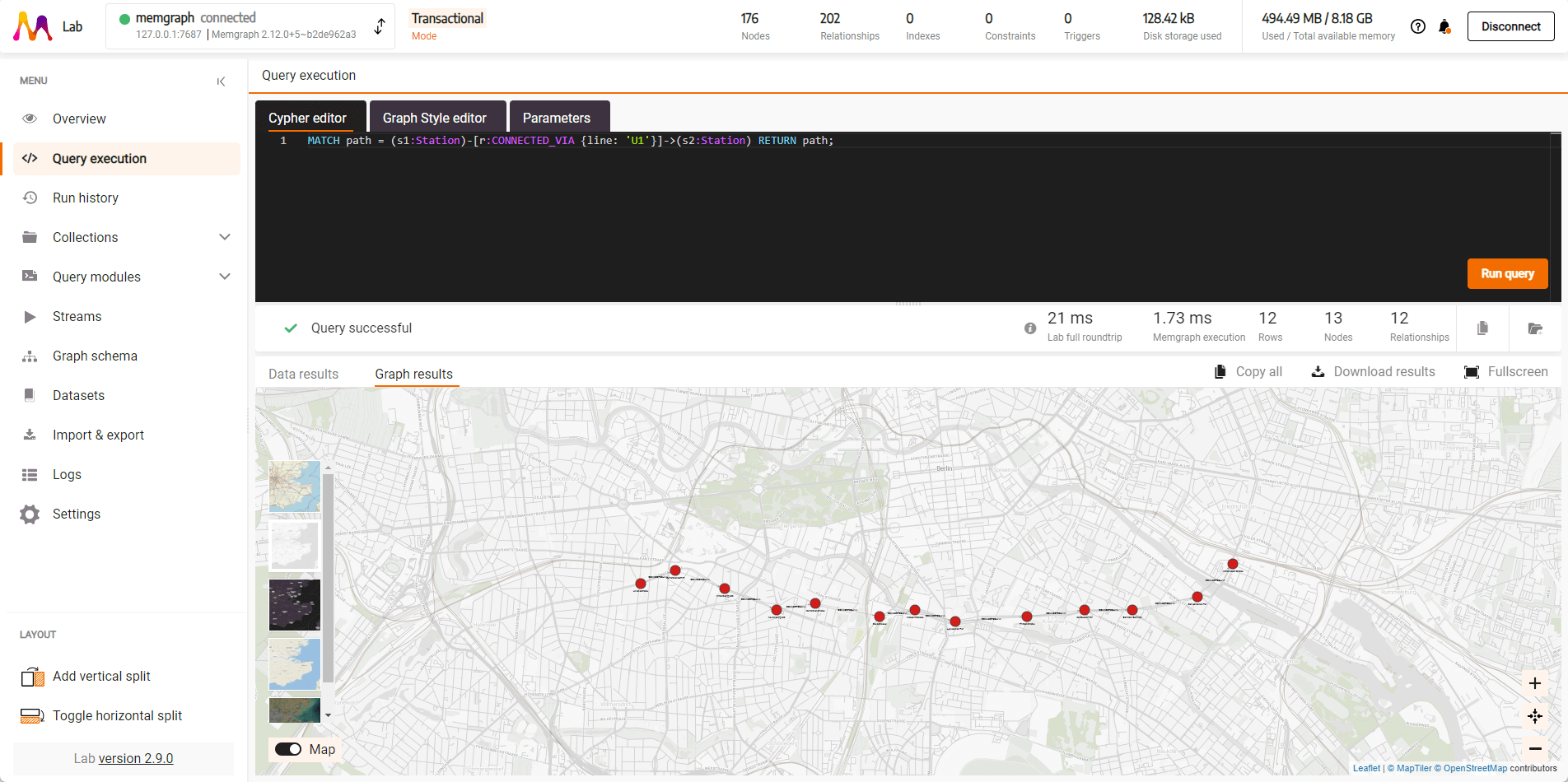
berlin subway all nodes If you want to see only one subway line, in this case, U1, use this query:

MATCH path = (s1:Station)-[r:CONNECTED_VIA {line: 'U1'}]->(s2:Station) RETURN path;

berlin subway u1 line

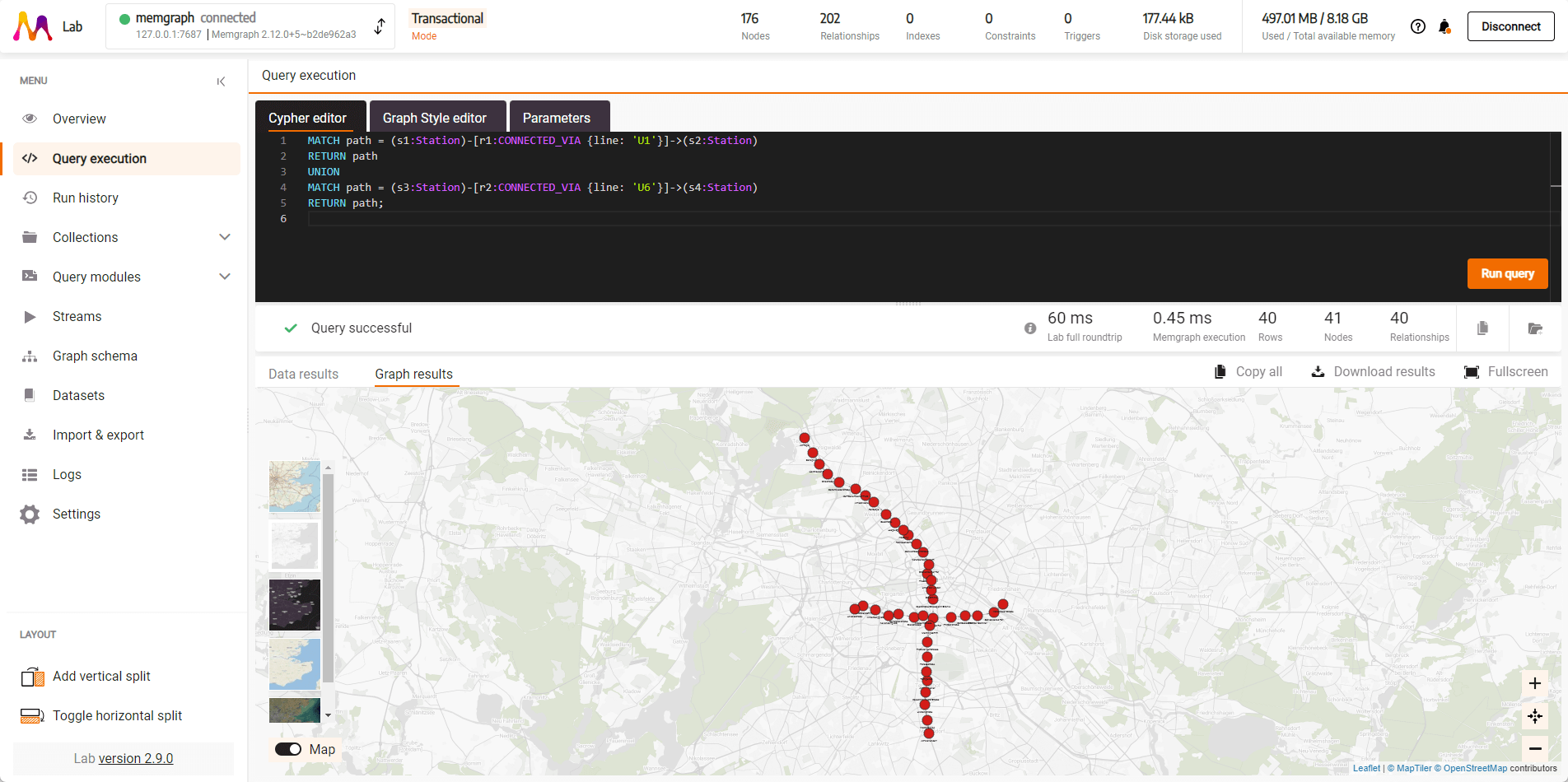
If you want to see two lines (U1 and U6) at the same time, run this query:

MATCH path = (s1:Station)-[r1:CONNECTED_VIA {line: 'U1'}]->(s2:Station)
RETURN path
UNION
MATCH path = (s3:Station)-[r2:CONNECTED_VIA {line: 'U6'}]->(s4:Station)
RETURN path;

berlin subway u1 u6 lines.png

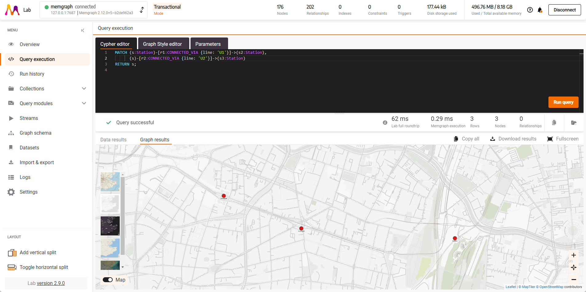
If you want to see which stations U1 and U6 have in common, run this query:

MATCH (s:Station)-[r1:CONNECTED_VIA {line: 'U1'}]->(s2:Station),
      (s)-[r2:CONNECTED_VIA {line: 'U2'}]->(s3:Station)
RETURN s;

berlin subway u1 u6 stations

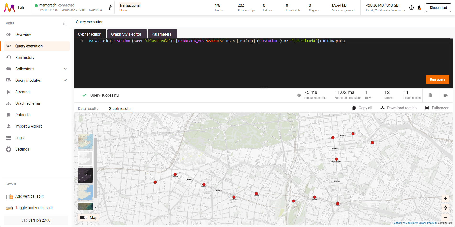
You can use algorithms, such as Weighted shortest path, to find the shortest path between two stations:

MATCH path=(s1:Station {name: "Uhlandstraße"})-[:CONNECTED_VIA *WSHORTEST (r, n | r.time)]-(s2:Station {name: "Spittelmarkt"}) RETURN path;

berlin subway shortest path

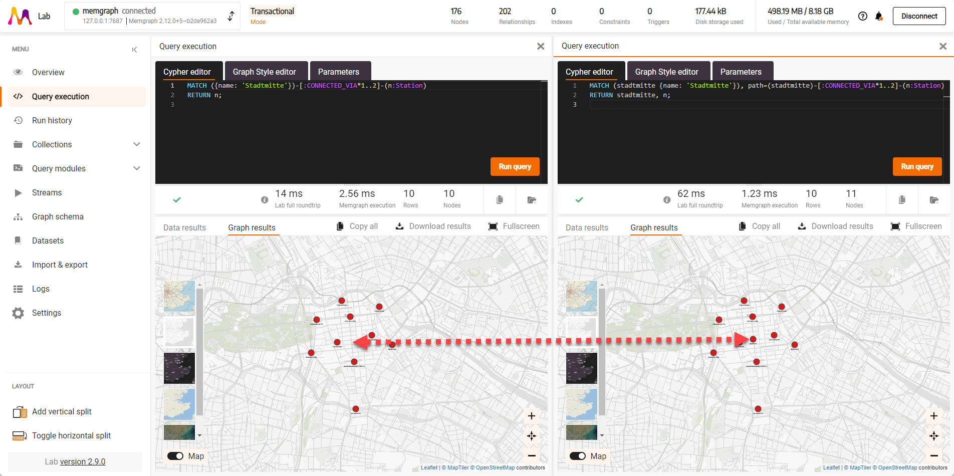
If you want to see what stations are up to two hops away from station Stadtmitte, you can run this query:

MATCH ({name: 'Stadtmitte'})-[:CONNECTED_VIA*1..2]-(n:Station)
RETURN n;

You will probably notice that the station Stadtmitte is not shown on the map. If you want to include it on the map, you need to modify the query a little bit:

MATCH (stadtmitte {name: 'Stadtmitte'}), path=(stadtmitte)-[:CONNECTED_VIA*1..2]-(n:Station)
RETURN stadtmitte, n;

berlin subway two hops

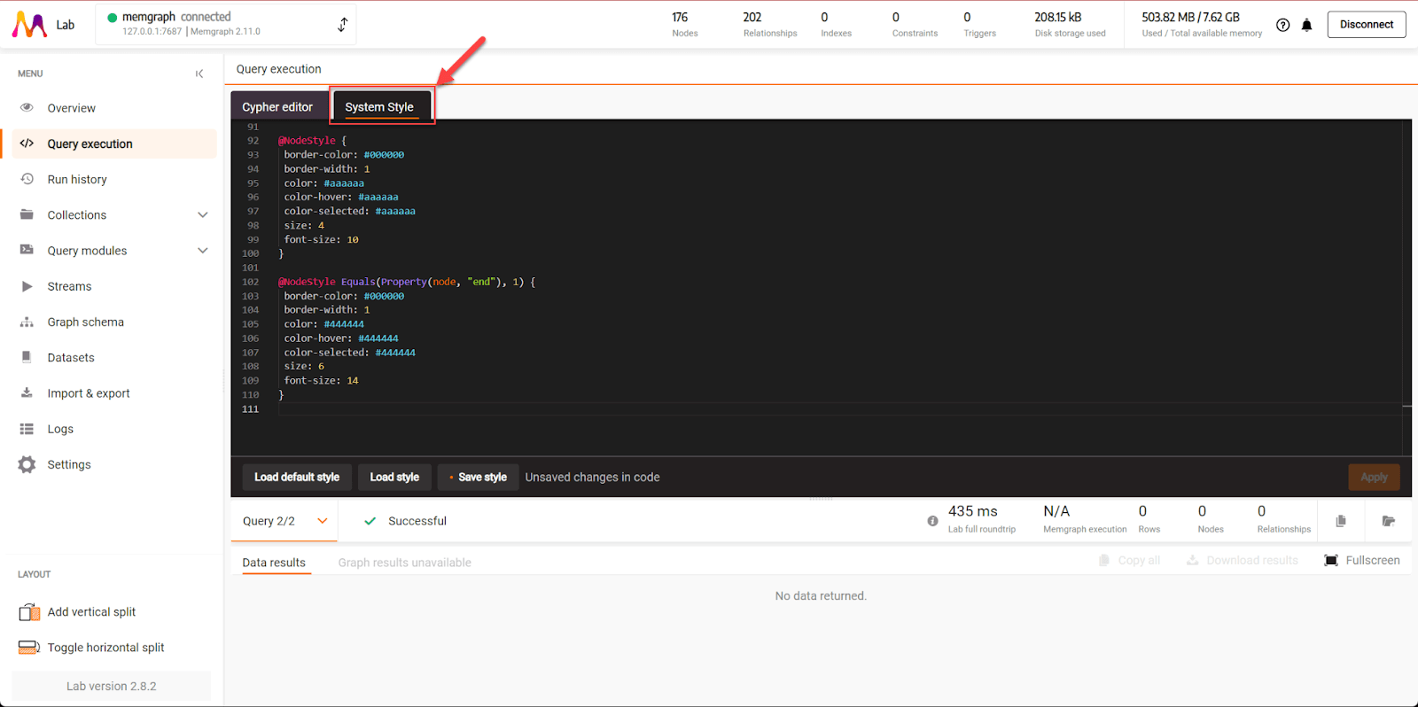
Add some flare to your graph: styling graphs

It is nice to see the data on the map, but with so many different lines it might be hard to see the connection between the stations that you are looking for. Let’s fix this by adding some colors to the data! First, let's make sure that all stations look the same, except for start and end stations. We’ll make those a little bit bigger. Open the Graph Style editor tab. Once you click on it, the tab name will change to the name of the style that is currently in use, System Style. We will use GSS code for graph styling. First, define all nodes to be gray (#aaaaaa), 4 pixels in size, and have labels of size 10. For start and end stations use a darker shade of gray (#444444), they will be 6 pixels and have labels of size 14.

Now, add the following code as the last lines of the code:

@NodeStyle {
 border-color: #000000
 border-width: 1
 color: #aaaaaa
 color-hover: #aaaaaa
 color-selected: #aaaaaa
 size: 4
 font-size: 10
}

@NodeStyle Equals(Property(node, "end"), 1) {
 border-color: #000000
 border-width: 1
 color: #444444
 color-hover: #444444
 color-selected: #444444
 size: 6
 font-size: 14
}

berlin subway two hops

While we are still in the editor, let’s add some color to the lines. On the Wikipedia page about Berlin subway I found the RAL color values for each of the nine lines. I’ve converted them to RGB values and I’ve assigned them to lines.

@EdgeStyle {
  label: Property(edge, "line")
  width: 4
  width-hover: 8
  arrow-size: 0
  font-size: 10
}

@EdgeStyle Equals(Property(edge, "line"), "U1") {
  color: #50C878 /* RAL 6018 */
  color-hover: #50C878
  color-selected: #50C878
}

@EdgeStyle Equals(Property(edge, "line"), "U2") {
  color: #D84B20 /* RAL 2002 */
  color-hover: #D84B20
  color-selected: #D84B20
}

@EdgeStyle Equals(Property(edge, "line"), "U3") {
  color: #317873 /* RAL 6016 */
  color-hover: #317873
  color-selected: #317873
}

@EdgeStyle Equals(Property(edge, "line"), "U4") {
  color: #FAD201 /* RAL 1023 */
  color-hover: #FAD201
  color-selected: #FAD201
}

@EdgeStyle Equals(Property(edge, "line"), "U5") {
  color: #885000 /* RAL 8007 */
  color-hover: #885000
  color-selected: #885000
}

@EdgeStyle Equals(Property(edge, "line"), "U6") {
  color: #9C7C8B /* RAL 4005 */
  color-hover: #9C7C8B
  color-selected: #9C7C8B
}

@EdgeStyle Equals(Property(edge, "line"), "U7") {
  color: #007AA5 /* RAL 5012 */
  color-hover: #007AA5
  color-selected: #007AA5
}

@EdgeStyle Equals(Property(edge, "line"), "U8") {
  color: #004547 /* RAL 5010 */
  color-hover: #004547
  color-selected: #004547
}

@EdgeStyle Equals(Property(edge, "line"), "U9") {
  color: #FF9500 /* RAL 2003 */
  color-hover: #FF9500
  color-selected: #FF9500
}

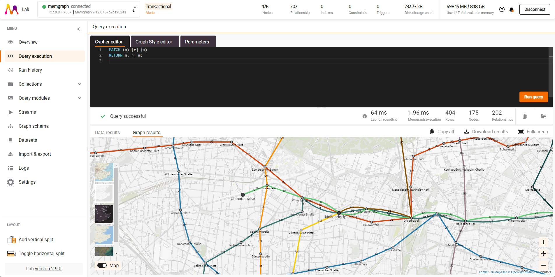
Save the style, and then run the following Cypher query to see the results:

MATCH (n)-[r]-(m)
RETURN n, r, m;

This doesn’t look bad, right?

berlin subway with style

Takeaway

Congratulations, you’ve just taken a deep dive into the world of graph databases and Memgraph Lab! You’ve learned how to import and visualize complex subway networks, run insightful queries, and style your results for maximum impact. These skills open up a world of possibilities for data analysis and visualization, and we encourage you to continue exploring and experimenting with Memgraph Lab. The subway network of Berlin is just the beginning—there are endless networks and connections out there waiting to be discovered and understood. Happy exploring!