Become an Inspector for a Day and Detect Fraudsters With Graph ML on Memgraph!

Whether you are an ML enthusiast or ML Expert, you probably heard of Graph Machine Learning. It is one of the most hyped and interesting branches of machine learning right now. As the name suggests, data in GraphML is represented by graphs. Graphs are easily stored in graph databases, and this is where our beloved in-memory database comes into play: Memgraph! We have already implemented a lot of famous graph algorithms through easy-to-use query modules. You can also read about our first Graph ML query module, the TGN query module.

This blog post deals with solving fraud detection problems with Graph ML. More precisely, one of the most common problems of Graph ML is Node Classification, and fraud detection is one of many areas where it can be applied.

Before tackling Graph ML, check out our already written resources Graph Neural Networks, Node Classification and Fraud Detection, so you can easily understand the following reads.

Relevant theory

Graph Machine Learning is a branch of machine learning based on graph data. Graphs consist of nodes that may have associated feature vectors, and edges, which again may or may not have feature vectors attached. In general machine learning, feature vectors are used to represent numeric or symbolic characteristics of an object, called features, in a mathematical, easily analyzable way.

Node Classification is a Graph ML problem where a neural network algorithm has to determine the labelling of samples (represented as nodes) by looking at the labels of their neighbours. It is motivated by homophily, literally "love of sameness," a sociological theory that similar individuals will move toward each other and act in a similar manner.

Algorithms learn from nodes’ feature vectors, while edges don’t need to have them attached. Therefore, nodes must have some feature vector attribute, but it is not always the case that publicly available graphs have them. Either case, we can always initialize them at random because of the expressive power of GNNs as “The surprising power of graph neural networks with random node initialization” paper suggests.

The easiest way for users to initialize feature vectors is by using the already existing query module: Node2Vec. That is a semi-supervised learning algorithm which learns feature vectors according to graph structure.

Fraud detection is a process that detects and prevents fraudsters from obtaining money or property through false means. Fraud detection is prevalent across banking, insurance, medical, government, and public sectors, as well as law enforcement agencies. Believe it or not, we can become inspectors and catch fraudsters with Node Classification! We can build and train a machine learning model based on a labeled training dataset we already have. Then we can use this trained model to predict the labels of a testing dataset which we have never encountered before - that’s the key: using previous experience, to detect fraudsters in the future! This process is called Inductive learning.

Research scientists have developed many successful Graph Neural Networks to tackle Inductive learning. Most common are Graph Attention Network (GAT) and GraphSAGE. They also developed GAT with Jumping Knowledge (GAT+JK) which showed one of the best performances with fraud detection datasets.

Let’s go on to the hot stuff - real world use cases!

Graph nodes and edges can optionally have a type. A graph with a single type of node and a single type of edge is called homogeneous. The first dataset we worked on is an example of a homogeneous graph: presenting Yelp Fraud dataset!

Yelp-Fraud dataset

It is now common practice for Web sites to enable their customers to write reviews of products they have purchased. Such reviews are valuable sources of information on these products. Potential customers use them before deciding to purchase a product to find the experience of other customers. They are also used by product manufacturers to identify product issues and to find competitive intelligence information about their competitors. Unfortunately, this importance of reviews also gives good incentive for spam, which contains false positive or malicious negative opinions.

Image 1: Some reviews from Yelp

Yelp-Fraud is a Multi-relational Graph Dataset for Yelp Spam Review Detection. Nodes of graph are reviews, and edges between them are these three relations: 1) R-U-R: reviews commented by same user; 2) R-S-R: reviews under the same product with the same star rating; 3) R-T-R: two reviews under the same product posted in the same month. For the sake of simplicity, this graph will be modeled in Memgraph database with single node type, and single edge type. Dataset is publicly available and can be found here. There are ~45k nodes and ~3.5M edges in it. Also, there is 14.5% of fraudulent reviews in the dataset. Therefore, the dataset is imbalanced, which is always the case with fraud detection datasets (fraudsters are always a minority).

Data loading

First of all, we used mgconsole to load the data, and we used Memgraph Lab to run queries and visualize graph schema and the results. Everything mentioned can be downloaded as the Memgraph Platform.

We preprocessed the dataset from YingtongDou/CARE-GNN GitHub repository (so you don’t need to), and converted it to the appropriate .cypherl format. Download the whole dataset file (huge dataset, about 700 MB), or light dataset file (about 20 MB).

Now, load the yelp.cypherl file from one of the following options.

Note: you might encounter issues when importing both datasets with Memgraph Lab. In that case, import it with mgconsole in terminal by running the statement below. Be patient, as it might take some time.

~ mgconsole < yelp.cypherl

Once the data is imported, run Memgraph Lab and generate a Graph Schema (enter the section with the same name from the menu on the left side). You should be able to see a single node type for reviews called :NODE and a single edge type for all sorts of connections called :EDGE (What a shocker ).

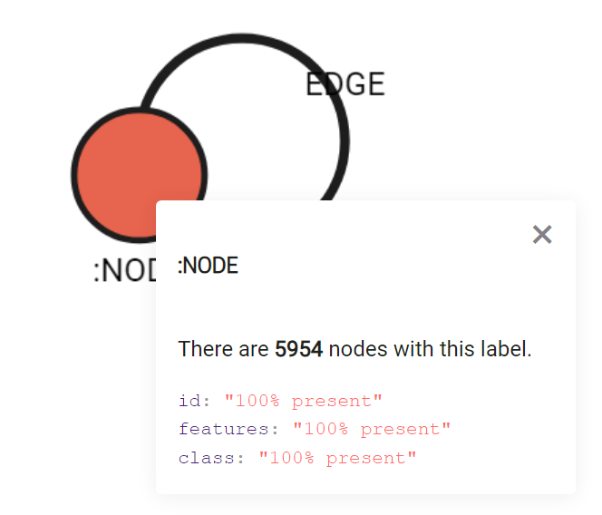
Image 2: Yelp Fraud light dataset graph schema. Nodes have properties id, features and class.

Since we are dealing with Inductive learning, we need nodes that the network has not already seen. We want to randomly split the dataset, save the smaller part of the dataset into a JSON file, run learning on the bigger part, then load the smaller part to make predictions. Let’s drop and return 100 random nodes with the following query:

MATCH (n)
WITH n, rand() AS r, n.id AS id, n.features AS features
ORDER BY r
LIMIT 100
DETACH DELETE n
RETURN id, features;

You can now click to “Download results” (on the right side of Memgraph Lab) to save them to a .json file.

Note: since this is a very huge dataset, you might run out of RAM while training (16 GB is not enough, it will probably work with 40 GB of RAM). You can still run training on our light dataset (20% of original dataset).

Model

Apart from data, the state-of-the-art model for this dataset is GAT + JK. The Knowledge layer added to the end of GAT helps solve the problem of reduced homophility as it is discussed in “New Benchmarks for Learning on Non-Homophilous Graphs” by Lim et al. We have implemented it on our network.

The important thing to say is that this model had the best performance dealing with this imbalanced dataset. Other models (GAT, GraphSage) would predict all samples to the dominant class.

Let's Get Ready For Training!!!🎉 🎉 🎉

Training

1. In order to initialize a model, you need to set parameters. The parameters we will be: “GAT+JK” for layer type, learning rate of 0.001, two hidden layers with sizes 16 (list [16,16]), and batch size of 1000:

CALL node_classification.set_model_parameters({layer_type: "GATJK", learning_rate: 0.001, hidden_features_size: [16,16], batch_size: 1000}) YIELD * RETURN *;

2. Start training of neural network:

CALL node_classification.train(1000) PROCEDURE MEMORY UNLIMITED YIELD *;

3. You can obtain training data with the following query, and see training and validation losses and metrics:

CALL node_classification.get_training_data() YIELD *;

4. You should now load previously dropped and saved nodes from the .json file, instructions are available on Memgraph docs, just change the path to the location of the JSON file:

CALL json_util.load_from_path("path/to/output.json")
YIELD objects
UNWIND objects AS o
CREATE (:NODE {id: o.id, last_name: o.features})
RETURN o.id;

5. From the previous output, choose one of IDs to predict on:

MATCH (n {id:SOME_ID_FROM_PREVIOUS_OUTPUT})
CALL node_classification.predict(n)
YIELD * RETURN predicted_class;

6. You can see the last 5 saved models in the user defined directory. That folder will be in the same directory where Memgraph was initialized.

Hmm, this is all clear, but how do we plot learning curves? Luckily, at this moment you can open a Jupyter notebook, connect to Memgraph, and fetch training data with GQLAlchemy.

For example, you can plot curves for loss with the following tiny piece of code:

from gqlalchemy import Memgraph
import matplotlib.pyplot as plt
memgraph = Memgraph("127.0.0.1", 7687)

results = memgraph.execute_and_fetch(
    """
    CALL node_classification.get_training_data() YIELD *;
    """
)

epochs, loss = [], []

for result in results:
    epochs.append(result['epoch'])
    loss.append(result['loss'])

plt.plot(epochs, loss, label="Loss")
plt.plot(epochs, val_loss, label = "Validation Loss")
plt.legend(loc="upper right")
plt.show()

Here is an example of those plots with different metrics:

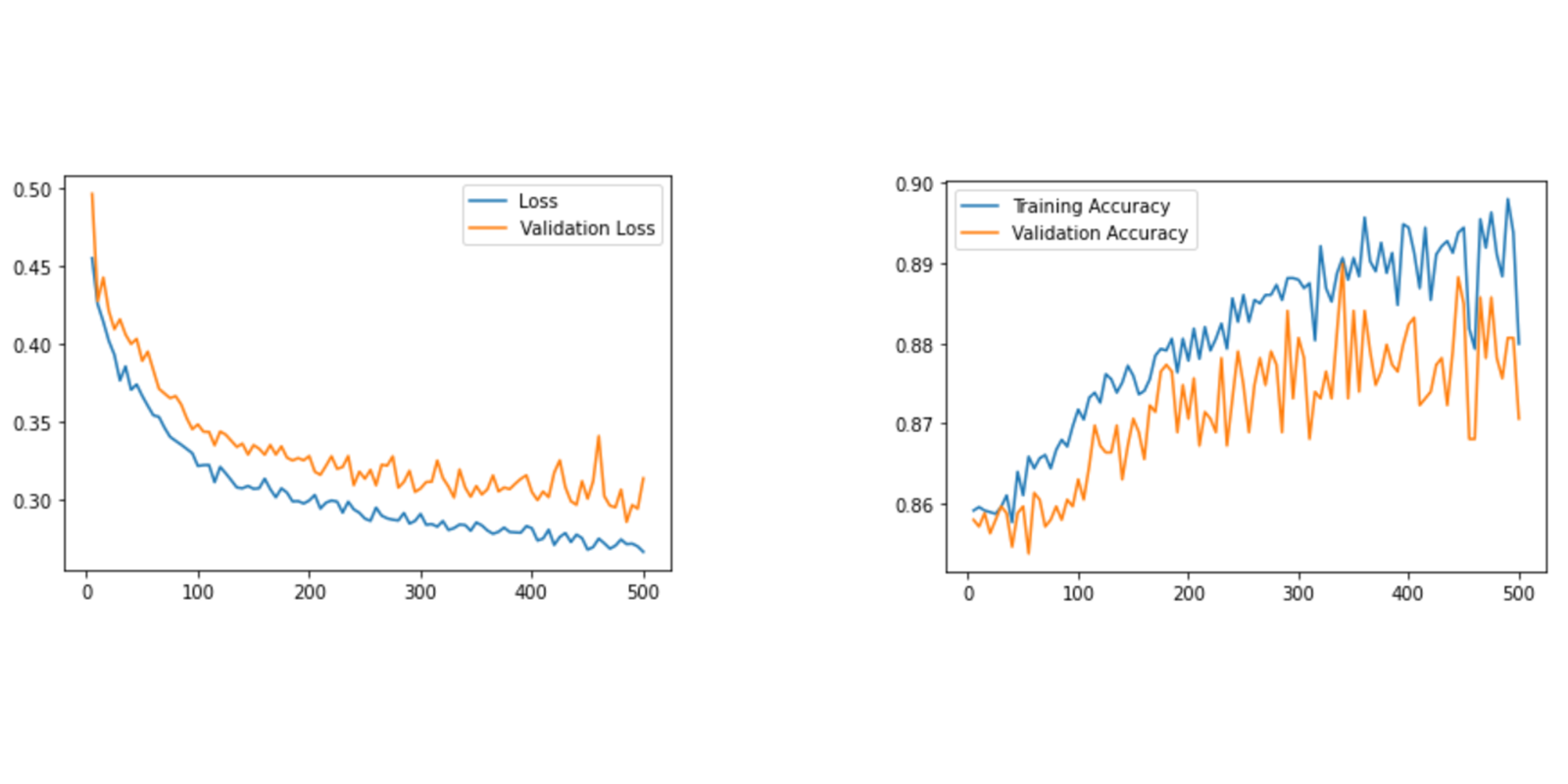
Image 3: Example of learning curves for losses and accuracies

Unfortunately, most graph datasets are not as simple as the previous example. Multiple nodes and edge types are much more common. Those graphs are called heterogeneous. On the other hand, there are not much publicly available hetero graph datasets for fraud detection. The main reason is that most companies tackling fraud detection have no interest in making datasets public.

Therefore, based on our experience with such systems, we created our very own heterogeneous graph dataset for fraud detection in insurance: home-made Artificial heterogeneous graph dataset, available on our memgraph/fraud-detection-use-case repository!

Artificial heterogeneous graph dataset

This dataset deals with insurances and detection of frauds at it. The most important nodes are those of type :CLAIM. An insurance claim is a formal request by a policy holder to an insurance company for coverage or compensation for a covered loss or policy event. Those nodes hold label fraud which indicates if the request was fraudulent or not. :CLAIM is agreed upon :INCIDENT and :CLAIM_PAYMENT is processed to those :INDIVIDUAL who requested it. :INDIVIDUAL experienced :INJURY, while contracted insurance :POLICY. :POLICY also insures a :VEHICLE, and it is contracted to some :ADRESS. Also, :INCIDENT is connected to some :POLICY, and happened to some :INDIVIDUAL. There will soon be a special blog post on how we constructed this dataset, so stay tuned!

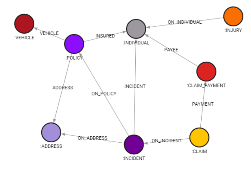
Image 4: hetero graph schema

You can generate your own .cypherl file following these steps:

~ git clone git@github.com:memgraph/fraud-detection-use-case.git
~ cd fraud-detection-demo/dataset
~ mkdir data
~ touch data/insurance.cypherl
~ python3 data_generator.py

It will fill data/insurance.cypherl file with Cypher queries, so you load it with:

~ mgconsole < data/insurance.cypherl

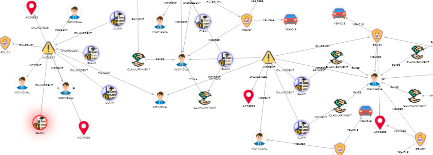
Image 5: subgraph of hetero graph with nice visuals

You can also execute the previous script with changed default parameters of total families and total incidents:

~ python3 data_generator.py <TOTAL_FAMILIES> <TOTAL_INCIDENTS>

where you change values <TOTAL_FAMILIES> and <TOTAL_INCIDENTS> to your preferences.

If you also want to have these nice visuals in Memgraph Lab, run

MATCH (n) RETURN n LIMIT 5;

enter Graph Style Editor, and paste the code from the dataset_style.gss file.

The first main difference is that this dataset doesn’t have feature vectors. This is a common thing in the industry, and it is always expected of data scientists to come up with their own features. As we explained before, the easiest way to form them is by using the existing query module Node2Vec. It sets the property “embedding” to each node:

CALL node2vec.set_embeddings() YIELD *;

Here, we will set different parameters, node properties for name of classes and features are different (class name is fraud, and feature vectors are now result embeddings from Node2Vec), and we change to lower batch size of 10:

CALL node_classification.set_model_parameters({layer_type: "GATJK", learning_rate: 0.001, hidden_features_size: [16,16], class_name: "fraud", features_name: "embedding", batch_size: 10}) PROCEDURE MEMORY UNLIMITED YIELD * RETURN *;

Before each training is executed, our code extracts features from nodes and concatenates them to matrices x, while :CLAIM also has labels and masks. Edge connections are stored in sparse matrices edge_index where the first dimension is always 2 (indicating node IDs which are connected).

The rest of the process now looks the same as before, we will provide only metrics. We performed this training on CUDA:

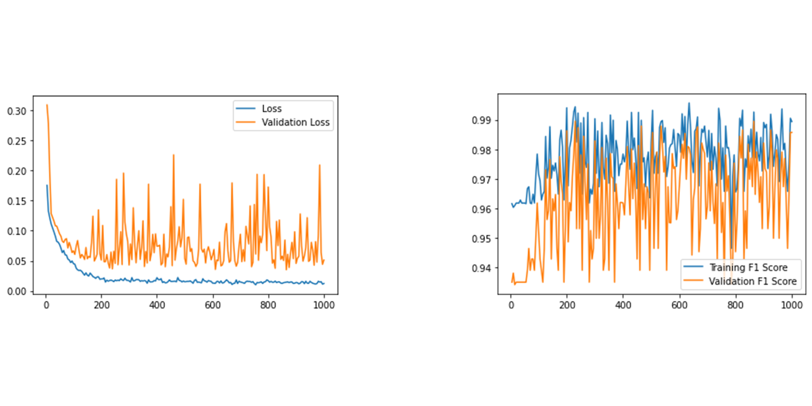
Image 6: Example of training losses and F1 Scores on hetero graph.

Conclusion

We have shown how graph machine learning can help solve fraud detection. We showed it in two examples, a homogeneous and a heterogeneous graph. This blog is intended as a headstart for someone who wants to deal with Graph ML. We hope this blog post will be helpful, and encourage you to train some models by yourself.