Temporal Graph Neural Networks With Pytorch - How to Create a Simple Recommendation Engine on an Amazon Dataset

April 26, 2022

Antonio Filipovic

PYTORCH x MEMGRAPH x GNN = 💟

Over the course of the last few months, we at Memgraph have been working on something that we believe could be helpful with classical graph prediction tasks. With our latest newborn query module, you will have the option of performing both label classification and link prediction.

But, how come a query module can do both label classification and link prediction? It's all thanks to graph neural networks, for short GNNs. ❤️

Graph neural networks

Whether you are a software engineer or a deep learning enthusiast, there is a high chance you heard of graph neural networks as a rising ⭐. Maybe you even deep-dived into this topic and are now ready for a new MAGE spell. But even if you haven't, don't worry, I will try to give you a quick overview so you can catch up and follow along.

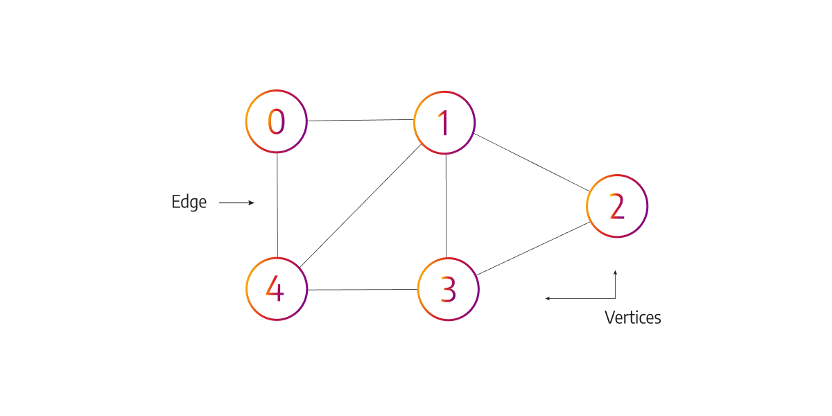
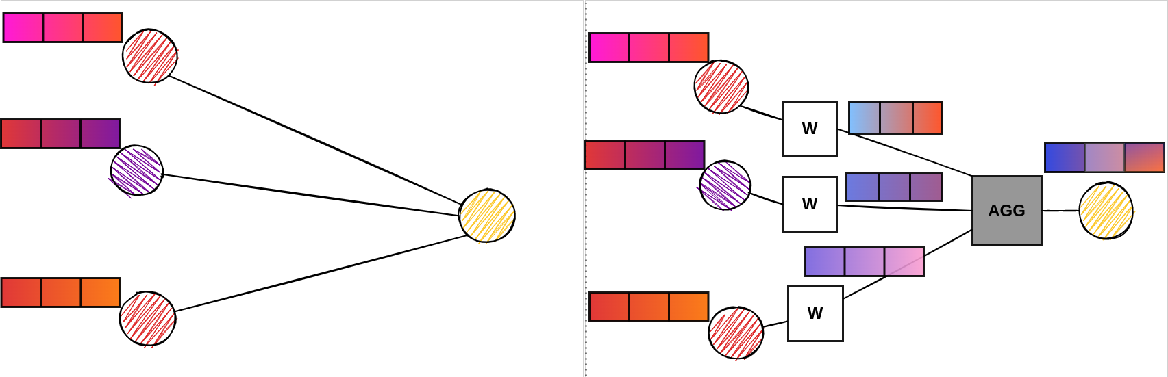
You probably already know that a graph consists of nodes (vertices) and edges (relationships). amazon-user-item-recommender-with-tgn-and-memgraph

Every node can have its feature vector, which essentially describes that node with a vector of numbers. We can look at this feature vector as the representation vector of each node, also called embedding of the node. To avoid getting lost in technical details, graph neural networks work as a message passing^[2] system, where each node aggregates feature representations of its 1-hop neighbors. To be more precise, nodes don’t aggregate feature representations directly, but feature vectors obtained by dimensionality reduction using the W matrix (you can look at them as fully connected linear layers). This matrix projected feature vectors are called messages and they give expressive power to graph neural networks.

amazon-user-item-recommender-with-tgn-and-memgraph

This idea originates from the field of graph signal processing. Now, we don't have time here to explain all about how we got from signals to message passing, but it's all math. Feel free to drop us a message on Discord and we will make sure to create a blog post explaining the graph neural network introduction topic, not a simplified version, but one explaining all of it from the beginning, somewhere about Tutorial on Spectral Clustering in 2007.

If you would like to get a better understanding of graph neural networks before continuing, I suggest you check out:

this blog post provides a gentle introduction to the topic
you can also check the video explanation by the Stanford professor Jure Leskovec about graph neural networks - I would honestly suggest to binge-watch the whole series, but if you don't have that much time, just watch the lectures called Message passing and Node Classification and Introduction to Graph Neural Networks
and if you want to deep-dive, which I suggest, I will leave the following blog post, it will be more than enough.

The reason why we added GNNs to MAGE is that GNNs are to graphs what CNNs are to images. GNNs can inductively learn about your dataset, which means that after training is complete you can apply their knowledge to a similar use case, which is very cool since you don't need to retrain the whole algorithm. With other representation learning methods like DeepWalk, Node2Vec, Planetoid, we haven't been able to do that until, well, GNNs.

Now, why temporal graph neural networks? Imagine you are in charge of a product where users interact with items every minute of every day, and they like some and hate the others. You would like to present them with more items they like, and not just that, you would love it if they bought those new items. This way you have a stream of data. Interactions appear across time, so you are dealing with a temporal dataset. The classical GNNs are not designed to work with streams, although they work very well on unseen data. But it is not all nails if you have a hammer - some methods work better on streams, others on static data.

Temporal graph networks

As you already know, we in Memgraph are all about streams.

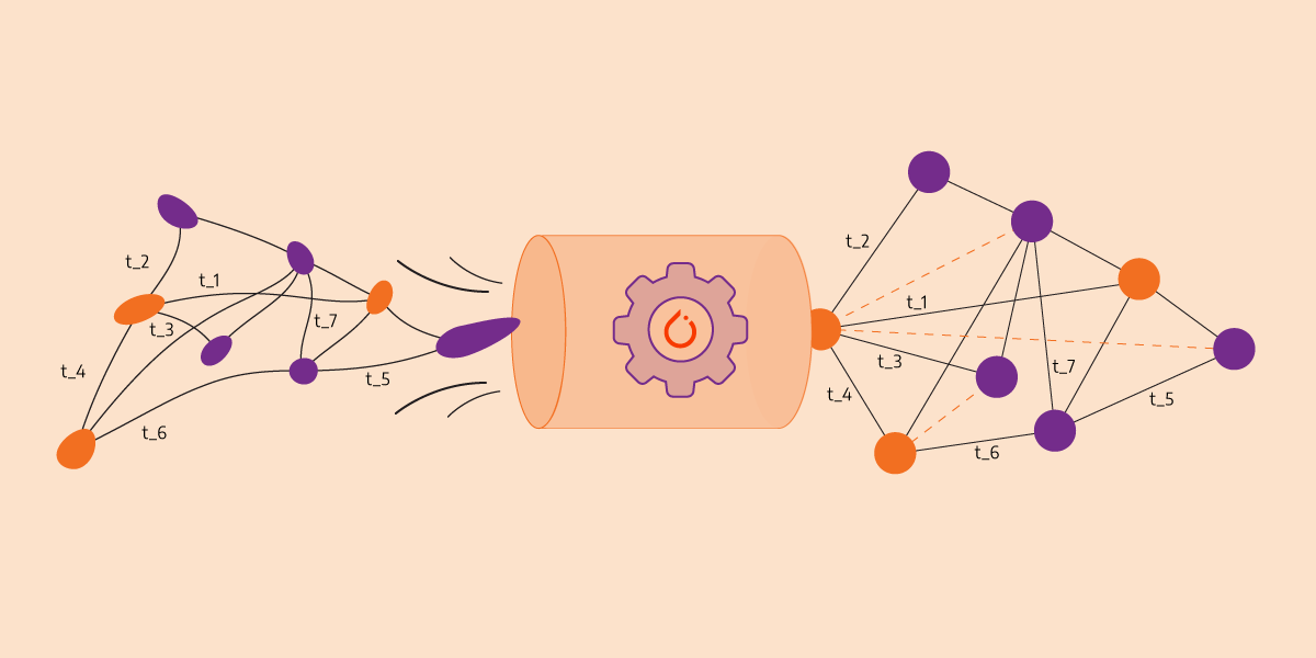
Thanks to the guys at Twitter, they developed a GNN that works on temporal graph networks. This way GNNs can deal with continuous-time dynamic graphs. In the image below you can see a schematic view of temporal graph networks. It is a lot to take in, but the process, once explained, is not that complicated.

Firstly, in continuous-time dynamic graphs, you can model changes on graphs that include edge or node addition, edge or node feature transformation (update), edge or node deletion as time-listed events.

Temporal graph networks^[1], shortened TGNs, work as follows:

node embedding calculations work on the concept of message passing, which I hope you are familiar with at this point
TGNs use events, and whenever a new edge appears, it represents an interaction event between two nodes involved
from every event, we create a message and use a message aggregator for all messages of the same node to get the aggregated message of every node
every node has its own memory which represents an accumulated state, updated with an aggregated message by one of the LSTM or GRU
Lastly, the embedding module is used to generate the temporal embedding

There are two embedding module types we integrated into our TGN implementation:

Graph attention layer: it is a similar concept as in Graph attention networks, but here they use the original idea from Vaswani et al. Attention is all you need which includes queries, keys and values and everything else is the same. I suggest you look at the TGN paper to check the exact embedding calculation details.
Graph sum layer: this mechanism is completely similar to the message passing system

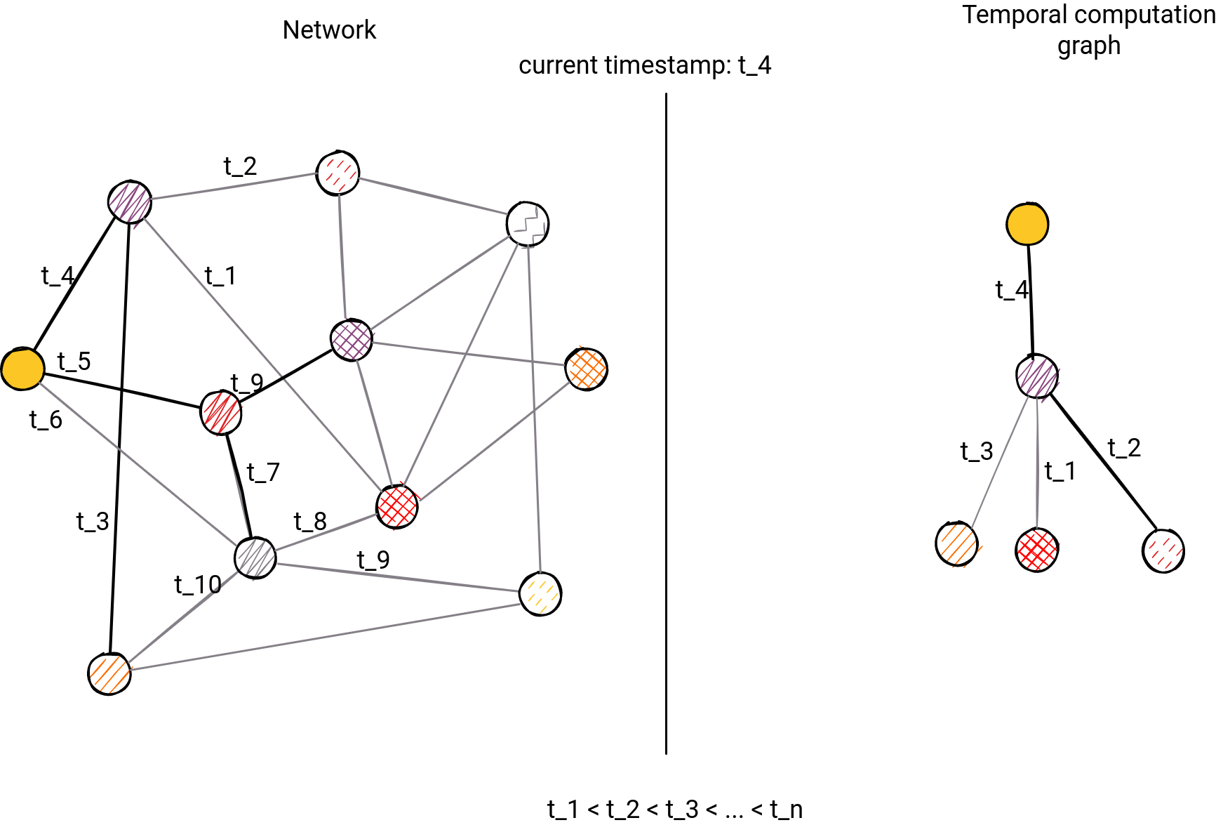
There is a certain problem when dealing with embedding updates. We don't update embeddings for every node, only for ones that appear in a batch. Also, in order not to get so much into implementation details, we will try to abstractly explain the following problem. Nodes in the batch appear at different points in time. That's why we need to take into account when was their update so that we can only use neighbors which appeared in the graph before them. This is in case we update the whole representation of the graph with batch information, and then do the calculation, which is what we did. This leads to having a different computation graph for every node. You can see what it looks like in the image below:

memgraph-temporal-computation-graph

Amazon data example

To try out how this works, we have prepared a Jupyter Notebook on our GitHub repository. It is about Amazon user-item reviews. In the following example, you will see how to do link prediction with TGN.

Exploring an Amazon data network in Memgraph

Through this short tutorial, you will learn how to install Memgraph, connect to it from a Jupyter Notebook and perform data analysis on an Amazon dataset using a graph neural network called Temporal graph networks.

1. Prerequisites

For this tutorial, you will need to install:

Docker is used because Memgraph is a native Linux application and cannot be installed on Windows and macOS.

2. Installation using Docker

After installing Docker, you can set up Memgraph by running:

docker run -it -p 7687:7687 -p 3000:3000 -p 7444:7444 memgraph/memgraph-platform

This command will start the download and after it finishes, run the Memgraph container.

3. Connecting to Memgraph with GQLAlchemy

We will be using the GQLAlchemy object graph mapper (OGM) to connect to Memgraph and execute Cypher queries easily. GQLAlchemy also serves as a Python driver/client for Memgraph. You can install it using:

pip install gqlalchemy

Hint: You may need to install CMake before installing GQLAlchemy.

Maybe you got confused when I mentioned Cypher. You can think of Cypher as SQL for graph databases. It contains many of the same language constructs like CREATE, UPDATE, DELETE... and it's used to query the database.

from gqlalchemy import Memgraph

memgraph = Memgraph("127.0.0.1", 7687)

Let's make sure that Memgraph is empty before we start with anything else.

memgraph.drop_database()

Following command should output {number_of_nodes:0}

results = memgraph.execute_and_fetch(
    """
    MATCH (n) RETURN count(n) AS number_of_nodes ;
    """
)
print(next(results))

4. Data analysis on an Amazon product dataset

You will load an amazon product dataset as a list of Cypher queries. This is what it looks like:

An example of the aforementioned queries is the following one:

MERGE (a:User {id: 'A1BHUGKLYW6H7V', profile_name:'P. Lecuyer'})
MERGE (b:Item {id: 'B0007MCVQ2'})
MERGE (a)-[:REVIEWED {review_text:'Like all Clarks, these guys didnt disappoint. They fit great and look even better. For the price, I dont think a better deal exists out there for casual shoes.',
  feature: [161.0, 133.0, 0.782608695652174, 0.0, 0.031055900621118012, 0.17391304347826086, 0.043478260869565216, 36.0, 36.0, 1.0, 3.6944444444444446, 0.0, 0.0, 3.0, 1.0, 12.0, 0.055, 0.519, 0.427, 0.9238],
  review_time:1127088000, review_score:5.0}]->(b);

So as you can see, we have User nodes and Item nodes in our graph schema. Every user has left a very positive review for an Item. This wasn't the case for all the reviews in our original dataset, but we processed it and removed negative reviews (all reviews with review_score <= 3.0). Every User has an id and every Item that has been reviewed has an id as well. In this one query, we find the User and the Item with mentioned ids or we create one if such User or Item is missing from the database. We create an interaction event between them in terms of an edge which has a list of 20 edge features. This edge_features we created from user reviews:

1. Number of characters
2. Number of characters without counting white space
3. Fraction of alphabetical characters
4. Fraction of digits
5. Fraction of uppercase characters
6. Fraction of white spaces
7. Fraction of special characters, such as comma, exclamation mark, etc.
8. Number of words
9. Number of unique works
10. Number of long words (at least 6 characters)
11. Average word length
12. Number of unique stopwords
13. Fraction of stopwords
14. Number of sentences
15. Number of long sentences (at least 10 words)
16. Average number of words per sentence
17. Positive sentiment calculated by VADER
# VADER - Valence Aware Dictionary and sEntiment Reasoner lexicon
# and rule-based sentiment analysis tool
18. Negative sentiment calculated by VADER
19. Neutral sentiment calculated by VADER
20. Compound sentiment calculated by VADER

We should have also prepared features for a User and Item, but these features seemed enough for our example.

One more note: In this dataset of queries we already prepared for you, there is one query that will change the "working mode" of our temporal graph networks module to evaluation(eval) mode. When the mode of the tgn is changed it also stops doing training of the model and starts doing evaluation of the trained model. If you look inside the file, you should find the following query:

CALL tgn.set_mode("eval") YIELD *;

Trigger creation

In order to process a dataset, we need to create a trigger on the edge create event if a trigger with that name doesn't exist.

This check is a neat feature to have in your Jupyter notebook if you want just to rerun it without dumping the local Memgraph instance if you are not working with Docker.

results = memgraph.execute_and_fetch("SHOW TRIGGERS;")
 
trigger_exists = False
for result in results:
    if result['trigger name'] == 'create_embeddings':
            print("Trigger already exists")
            trigger_exists = True
            break;
 
 
if not trigger_exists:
    memgraph.execute(
        """
        CREATE TRIGGER create_embeddings ON --> CREATE BEFORE COMMIT
        EXECUTE CALL tgn.update(createdEdges) RETURN 1;
        """
    )

Index creation for dataset

Memgraph works best with indexes defined for nodes. In our case, we will create indexes for User and Item nodes.

index_queries = ["CREATE INDEX ON :User(id);",
                "CREATE INDEX ON :Item(id);"]
 
for query in index_queries:
    results = memgraph.execute_and_fetch(query)
    for result in results:
        continue

Training and evaluating Temporal Graph Networks

In order to train a Temporal graph network on an Amazon dataset, we will split the dataset into train and eval queries. Let's first load our raw queries. Each query creates an edge between User and Item thus representing a positive review of a certain Item by a User.

import os
 
dir_path = os.getcwd()
 
with open(f"{dir_path}/data/queries.cypherl", "r") as fh:
    raw_queries = fh.readlines()
 
train_eval_split_ratio = 0.8
queries_index_split = int(len(raw_queries) * train_eval_split_ratio)
 
train_queries = raw_queries[:queries_index_split]
eval_queries = raw_queries[queries_index_split:]
 
print(f"Num of train queries {len(train_queries)}")
print(f"Num of eval queries {len(eval_queries)}")

Before we start importing train queries, first we need to set parameters for temporal graph networks.

# since we are doing link prediction, we use self_supervised mode
learning_type = "self_supervised"
batch_size = 200 #optimal size as defined in paper
num_of_layers = 2 # GNNs don't need multiple layers, contrary to CNNs.
layer_type = "graph_attn" # choose between graph_attn or graph_sum
edge_message_function_type = "identity" # choose between identity or mlp
message_aggregator_type = "last" # choose between last or mean
memory_updater_type = "gru" # choose between gru or rnn
attention_heads = 1
memory_dimension = 100
time_dimension = 100
num_edge_features = 20
num_node_features=100
# number of sampled neighbors
num_neighbors = 15
# message dimension must be defined in the case we use MLP,
# because then we define dimension of **projection**
message_dimension = time_dimension + num_node_features + num_edge_features
 
tgn_param_query = f"CALL tgn.set_params({{learning_type:'{learning_type}',
batch_size: {batch_size}, num_of_layers:{num_of_layers},
layer_type:'{layer_type}', memory_dimension:{memory_dimension},
time_dimension:{time_dimension}, num_edge_features:{num_edge_features},
num_node_features:{num_node_features}, message_dimension:{message_dimension},
num_neighbors:{num_neighbors},
edge_message_function_type:'{edge_message_function_type}',
message_aggregator_type:'{message_aggregator_type}',
memory_updater_type:'{memory_updater_type}',
attention_heads:{attention_heads}}})
YIELD *;"
 
print(f"TGN param query: {tgn_param_query}")
 
results = memgraph.execute_and_fetch(tgn_param_query)
for result in results:
    print(result)

Now it is time to execute queries and perform the first epoch of training.

for query in train_queries:
    results = memgraph.execute_and_fetch(query.strip())
    for result in results:
        continue

Now we need to change TGN mode to eval and start importing our evaluation queries.

results = memgraph.execute_and_fetch("CALL tgn.set_eval() YIELD *;")
for result in results:
    print(result)
 
for query in eval_queries:
    results = memgraph.execute_and_fetch(query.strip())
    for result in results:
        continue

After our stream is done, we should probably do a few more rounds of training and evaluation in order to have a properly working model. We can do so with the following query:

num_of_epochs = 5
 
results = memgraph.execute_and_fetch(
    f"""
    CALL tgn.train_and_eval({num_of_epochs}) YIELD *
    RETURN epoch_num, batch_num, precision, batch_process_time, batch_type
    ORDER BY epoch_num, batch_num;
    """
)
 
for result in results:
    continue

Now, let's get the results and then do some plotting to check whether the precision increases between epochs.

from collections import defaultdict
import matplotlib.pyplot as plt
import numpy as np
 
results_train_dict = defaultdict(list)
results_eval_dict = defaultdict(list)
 
results = memgraph.execute_and_fetch(
    """
        CALL tgn.get_results()
        YIELD  epoch_num, batch_num, precision, batch_process_time, batch_type
        RETURN epoch_num, batch_num, precision, batch_process_time, batch_type
        ORDER BY epoch_num, batch_num;
    """
)
 
for result in results:
    if result['batch_type'] == 'Train':
        results_train_dict[result['epoch_num']].append(result['precision'])
    else:
        results_eval_dict[result['epoch_num']].append(result['precision'])

Now that we have collected the results, let's first plot the average accuracy of train batches inside epoch, and the average accuracy of eval batches inside epoch. We can do that since every batch is the same size. (NB: TGN uses a predefined batch size.)

X_train = []
Y_train = []
 
for epoch, batches_precision in results_train_dict.items():
    Y_train.append(np.mean(batches_precision))
    X_train.append(epoch)
 
X_eval = []
Y_eval = []
for epoch, batches_precision in results_eval_dict.items():
    Y_eval.append(np.mean(batches_precision))
    X_eval.append(epoch)
 
 
#scatter plot
plt.plot(X_train, Y_train, 'b', label="train")
plt.plot(X_eval, Y_eval, 'r', label="eval")
 
#add title
plt.title('epoch - average batch precision')
 
#add x and y labels
plt.xlabel('epoch')
plt.ylabel('precision')
plt.legend(loc="upper left")
 
#show plot
plt.show()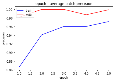

memgraph-average-batch-precision

We can see that average accuracy increases, which is really good. Now we can start creating some recommendations. Let's find Users who reviewed one Item positively and those who reviewed multiple Items positively. Our module will return what it believes should be a prediction score for yet unreviewed Items.

results = memgraph.execute_and_fetch(
    """
        MATCH (n:User)
        WITH n
        LIMIT 15
        MATCH (m:Item)
        OPTIONAL MATCH (n)-[r]->(m)
        WHERE r is null
        CALL tgn.predict_link_score(n,m) YIELD prediction
        WITH n,m, prediction
        ORDER BY prediction DESC
        LIMIT 10
        MERGE (n)-[:PREDICTED_REVIEW {likelihood:prediction}]->(m);
 
    """
)
for result in results:
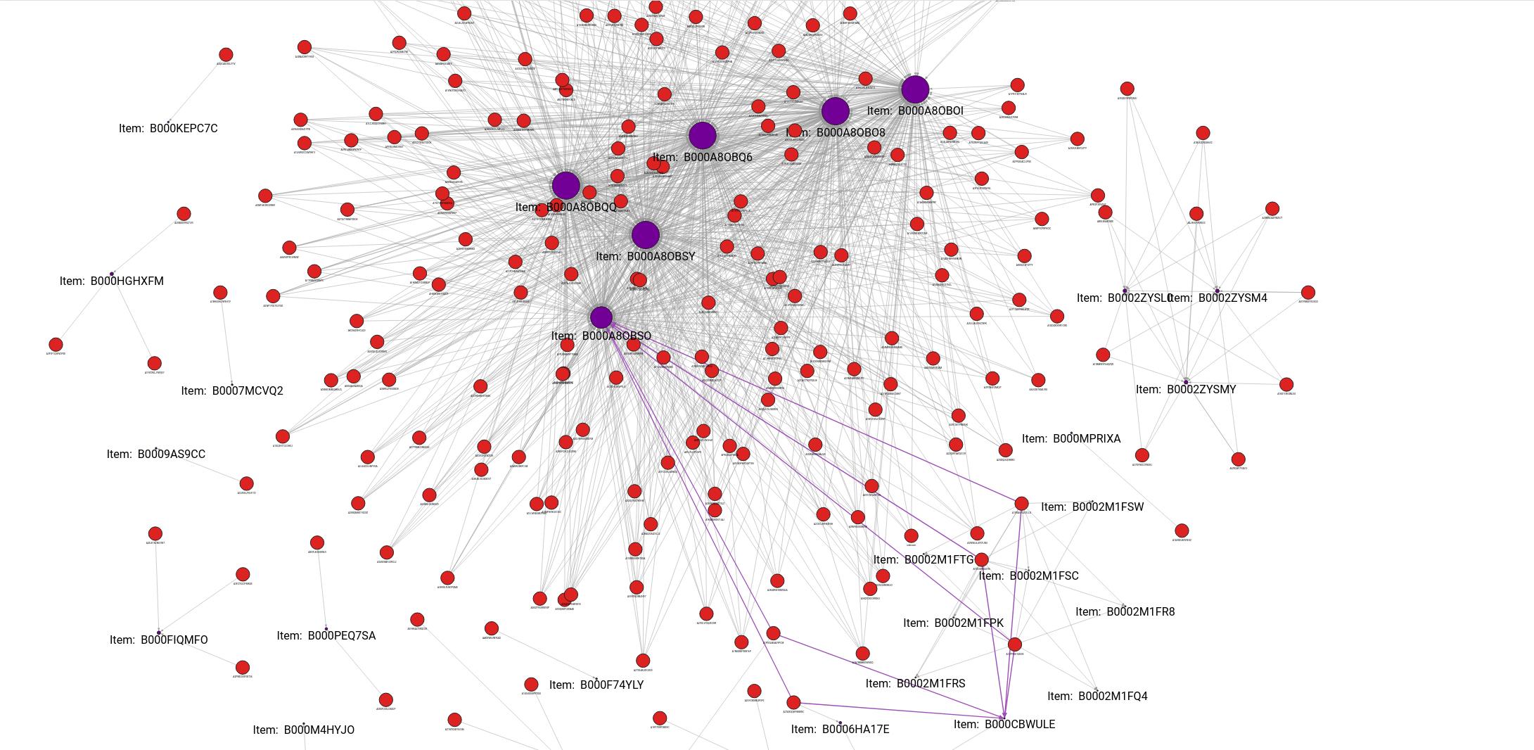
    print(result)

Now we can run the following query in Memgraph Lab:

MATCH (u:User)-[pr:PREDICTED_REVIEW]->(i:Item), (u)-[r:REVIEWED]->(oi:Item)
RETURN *;

And after applying a style, we get the following visualization. From the image below, we can see that most predictions are oriented towards one of the most popular items.

Where to next?

Well, I hope this was fun and that you have learned something. You can check out everything else that we implemented in the MAGE 1.2 release. If you loved our implementation, don't hesitate to give us a star on GitHub ⭐. If you have any comments or suggestions, you can contact us on Discord. And lastly, if you wish to continue reading posts about graph analytics, check out our blog.

References

[1] E. Rossi, B. Chamberlain, F. Frasca, D. Eynard, F. Monti, M. Bronstein (2020). Temporal Graph Networks for Deep Learning on Dynamic Graphs

[2] W.L. Hamilton, R. Ying, and J. Leskovec. Inductive representation learning on large graphs. U Advances in Neural Information Processing Systems 30, 2017