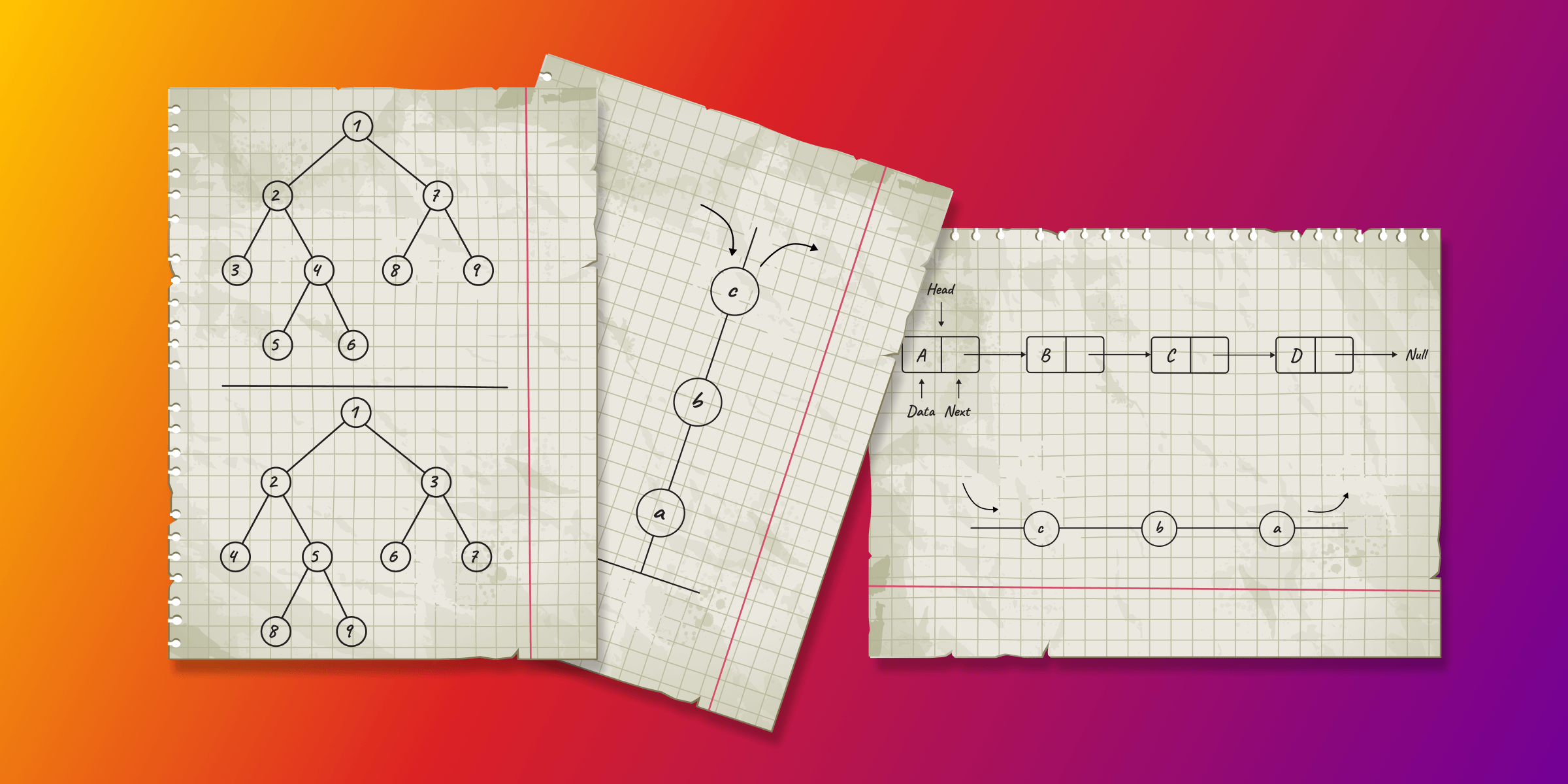
Data Structures Cheat Sheet

In this article, we will provide an introduction to data structures, offering examples of each structure and illustrating how they could be represented in Memgraph. Among these structures, graphs stand out as non-linear data structures composed of a finite set of nodes, connected by relationships. They are used to tackle real-world problems in areas such as networks, knowledge graphs or fraud detection cases.

Check out our infographic Data Structures Cheat Sheet for a quick reference on the structures we’ll discuss below.

What is a graph?

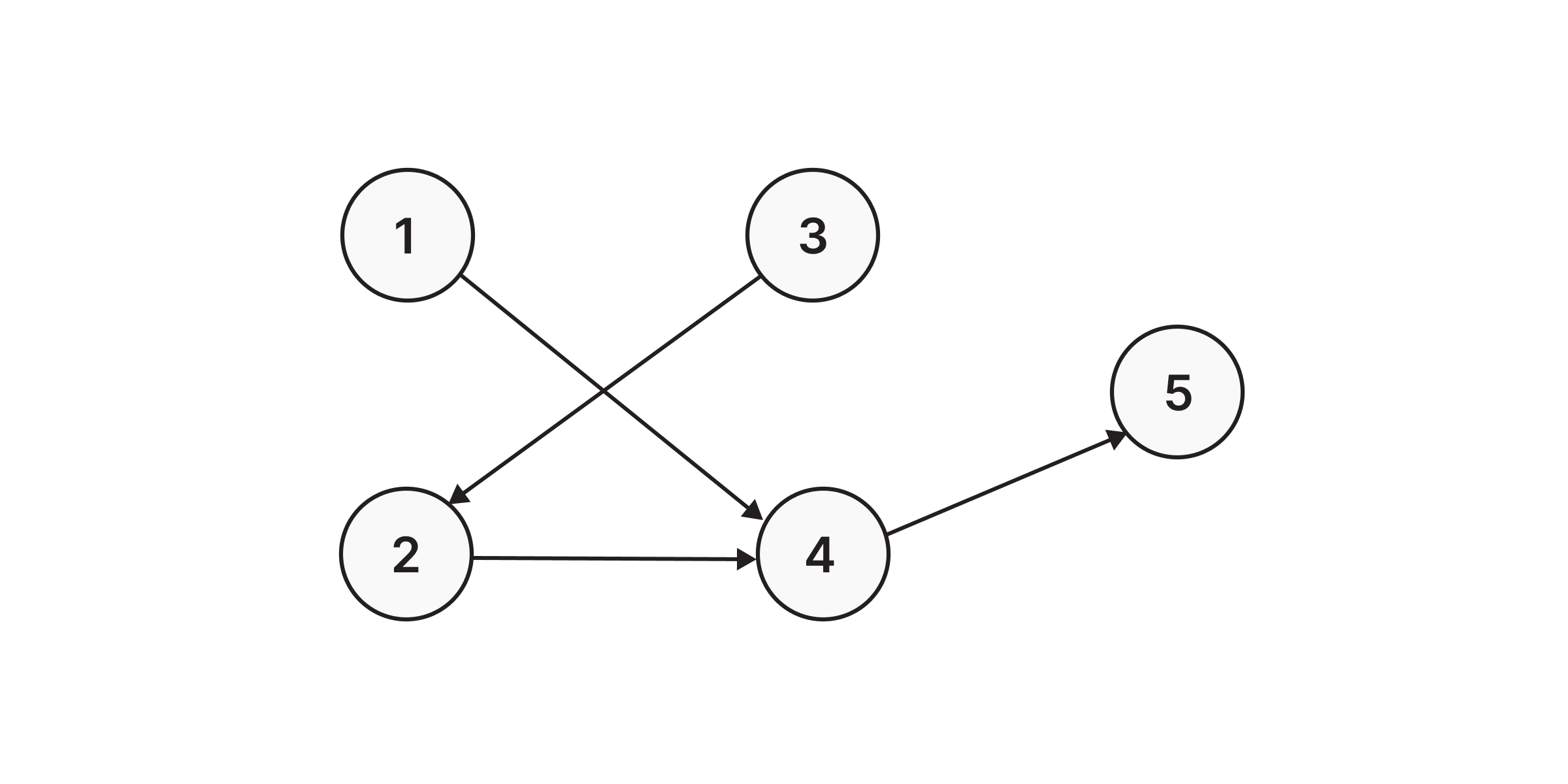
In order to dive into the world of data structures, it’s important to, first of all, get familiar with the basics. As already mentioned, a graph is a data structure made up of nodes (vertices) and relationships (edges). The relationships connect any two nodes in the graph, which can store different types of properties. In the picture below we can see a graph made out of five nodes connected with directed relationships.

Creating nodes and relationships

Let’s now create the graph from the picture above in Memgraph. Make sure you have a running Memgraph instance. If you haven’t yet installed Memgraph, visit our documentation guide for the installation instructions. The quickest way to try out Memgraph Platform (Memgraph database + MAGE library + Memgraph Lab) is by running one of the following commands with Docker running in the background:

For Linux/macOS:

curl https://install.memgraph.com | sh

For Windows:

iwr https://windows.memgraph.com | iex

From the picture above, we can see that we have five nodes, each marked with a certain number. Let’s create nodes such that the label is Node and numbers are name properties inside the node along with directed relationship :TO between them:

CREATE (n1:Node {name: '1'}), (n2:Node {name: '2'}),
(n3:Node {name: '3'}), (n4:Node {name: '4'}), (n5:Node {name: '5'}),
(n1)-[:TO]->(n4), (n3)-[:TO]->(n2),
(n2)-[:TO]->(n4), (n4)-[:TO]->(n5)

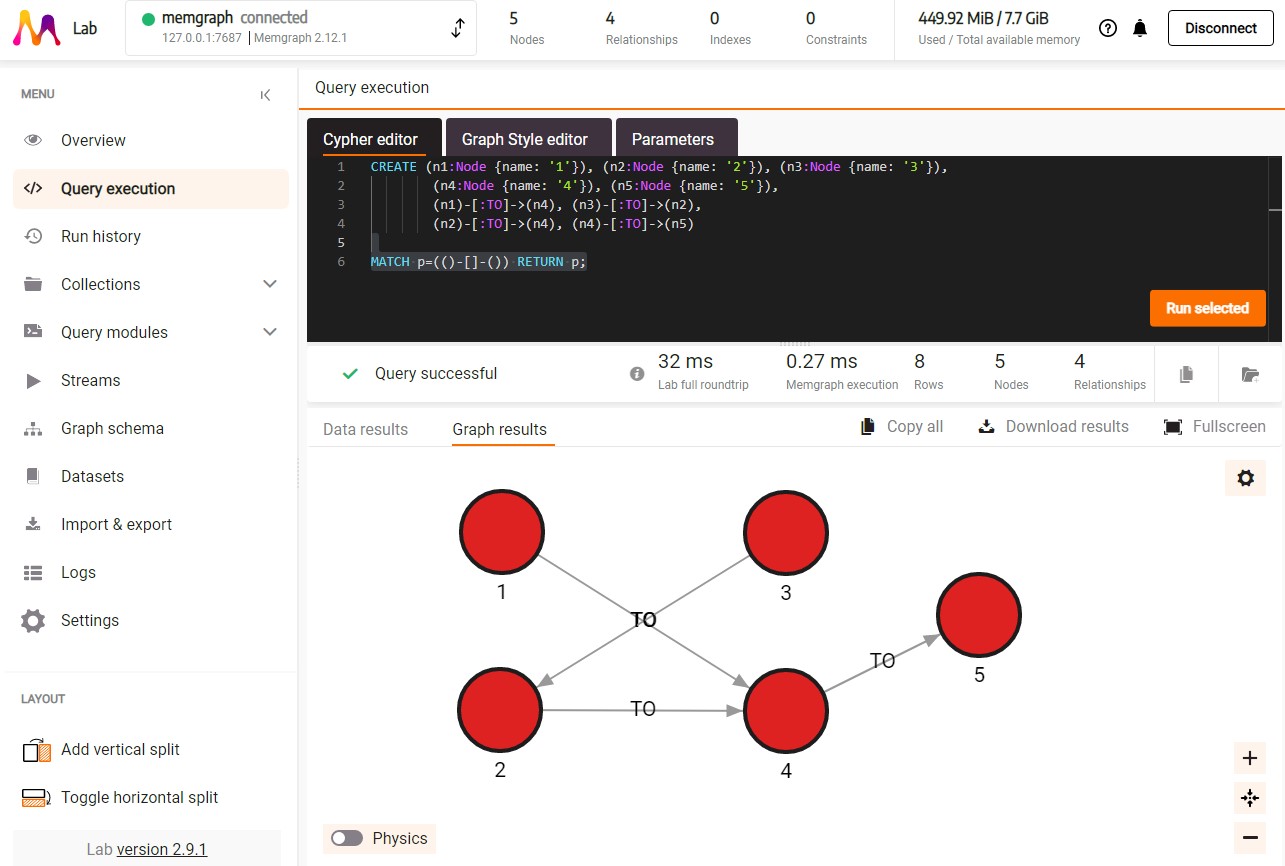
If you’re using Memgraph’s visual interface, Memgraph Lab, you’ll be able to see the visualization of your newly created graph by running

MATCH p=(()-[]-()) RETURN p;

Creating indexes

Just like hash functions have indexes, Memgraph also has the ability to create indexes on certain Node or Node+Property combinations in order to scan through the database and retrieve nodes faster when you have a larger dataset. In the example shown previously, it would make sense to create an index on the Node label if we had multiple different labels and a large dataset. Here’s an example of how to create an index on the Node label:

CREATE INDEX ON :Node

Data structures

In computer science, a data structure is a data organization, management and storage format that is usually chosen for efficient access to data. More precisely, a data structure is a collection of data values, the relationships among them, and the functions or operations that can be applied to the data. There are numerous types of data structures and in this article, we will mention a Linked List, Matrix, Queue, Stack and Tree Structure.

Linked List

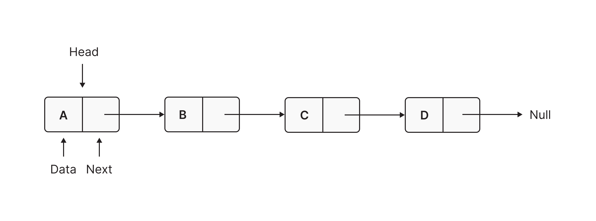
A linked list is a linear data structure, in which elements are not stored at a contiguous location, rather they are linked using pointers. It organizes items sequentially, with each item storing a pointer to the next one. An item in a linked list is called a node. The first node is called the head. The last node is called the tail.

Representing a Linked List in Memgraph

Similarly, in Memgraph we are also going to represent items in the linked list as nodes, but here we don’t have to store the information about the address of the next node, we can just use a directed graph in order for it to do it for us: Let's recreate the linked list from the image above. With relationship LINKED_TO:

CREATE (n1:Node {name: 'A'}), (n2:Node {name: 'B'}), (n3:Node {name: 'C'}), (n4:Node {name: 'D'}),
        (n1)-[:LINKED_TO]->(n2)-[:LINKED_TO]->(n3)-[:LINKED_TO]->(n4)

You can also store any additional properties inside your nodes, like IDcode>, different names of the nodes or any additional info.

By running the following query we will be able to visualize created data and easily access its properties by clicking on a certain node:

MATCH p=(()-[]-()) RETURN p;

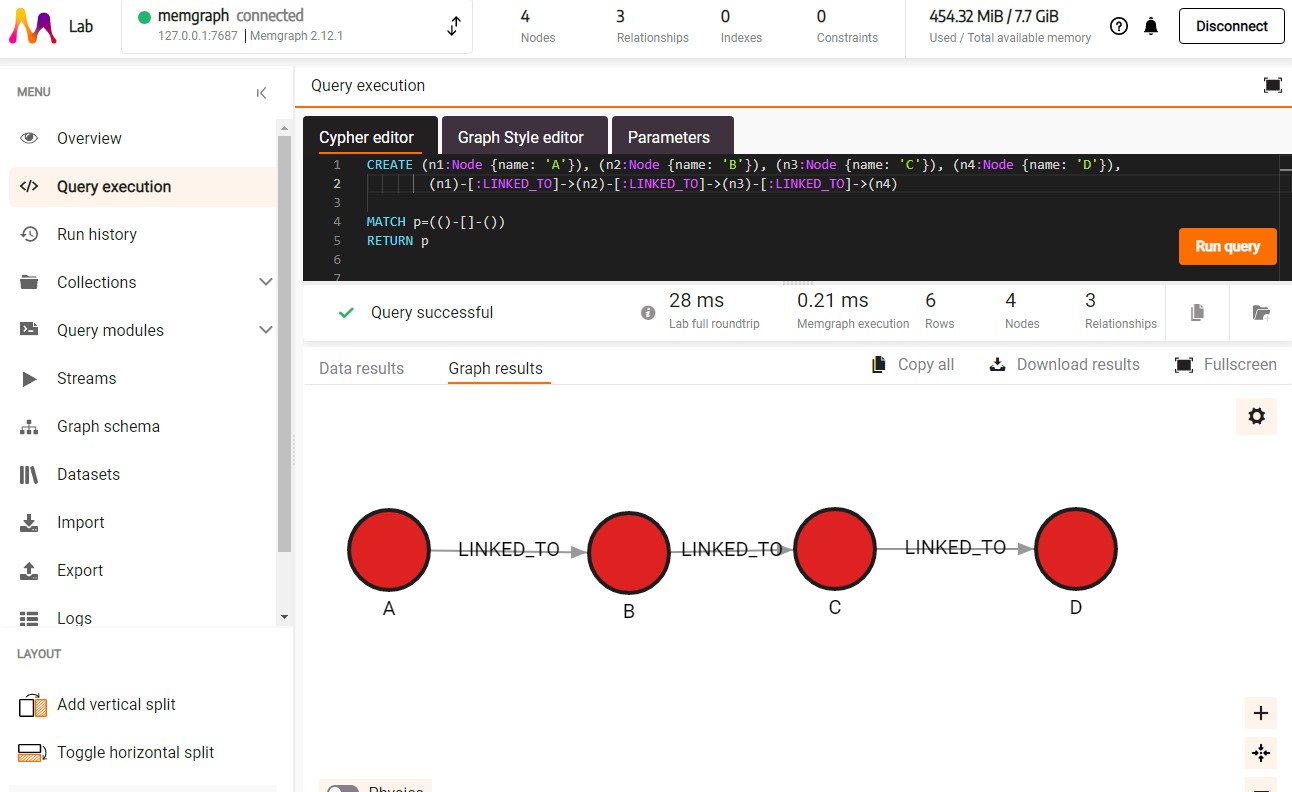
If you have a larger graph that is harder to visualize and want to, for example, retrieve information about where does the node named C link to, you can achieve it with this query:

MATCH (:Node {name: 'C'})-[:LINKED_TO]->(m)
RETURN m

Queue

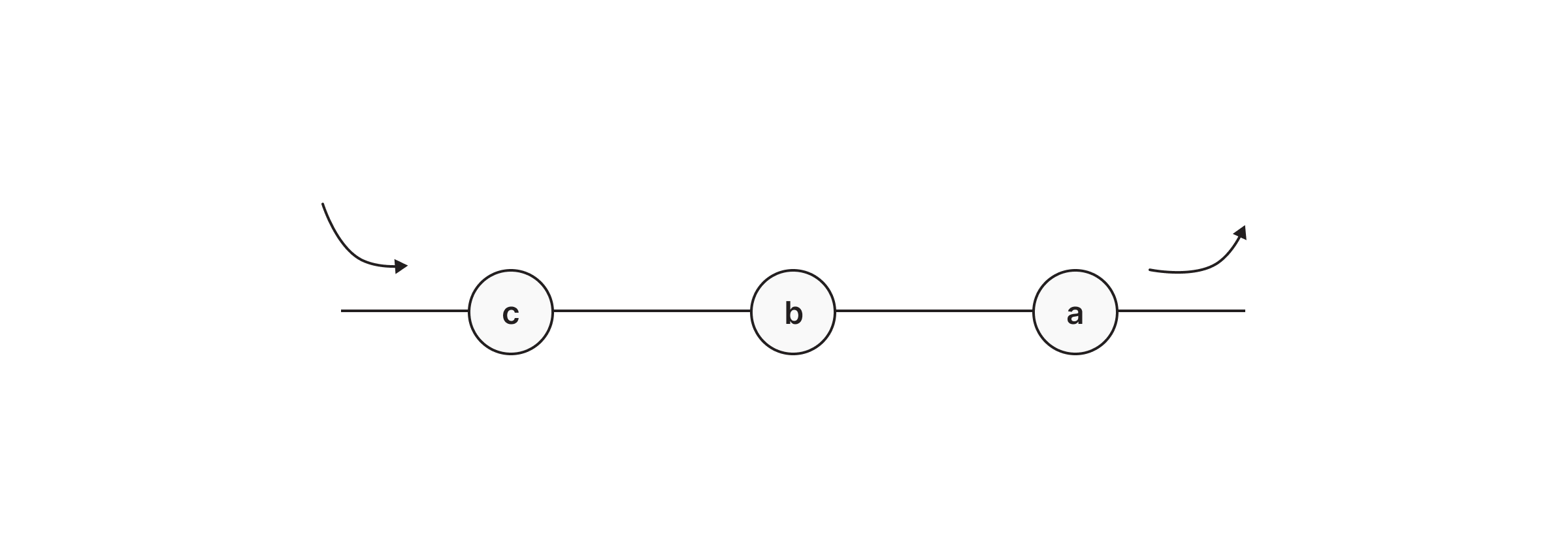
A Queue is a linear data structure that is open at both ends and the operations are performed in First In First Out (FIFO) order.

We define a queue to be a list in which all additions to the list are made at one end and all deletions from the list are made at the other end. The element that is first pushed into the order, the operation is first performed on that.

Representing a Queue in Memgraph

In Memgraph, we can represent a queue by simply creating nodes and connecting them with a relationship indicating which node came before with the :BEFORE relationship. Similarly, we can also create an :AFTER relationship and direct our relationships the other way around, depending on what suits us the best at the moment.

The following query creates three nodes and :BEFORE relationship between them, indicating that node A “came to the queue” first, followed by nodes B and C

CREATE (n1:Node {name: 'A'}), (n2:Node {name: 'B'}), (n3:Node {name: 'C'}),
(n1)-[:BEFORE]->(n2)-[:BEFORE]->(n3)

Operations with Queue

If we want to find out which element is in the front of the queue and remove it, similar to the Dequeue() function, we can do that with the following query:

MATCH (a)-[:AFTER]->(b)
WHERE NOT exists((b)-[:AFTER]->())
RETURN b

Similarly, if we want to add an element D to the end of the queue, mimicking the Enqueue() function:

MATCH (a)-[:AFTER]->(b)
WHERE NOT exists(()-[:AFTER]->(a))
CREATE (n4:Node {name: 'D'})-[:AFTER]->(a)

Stack

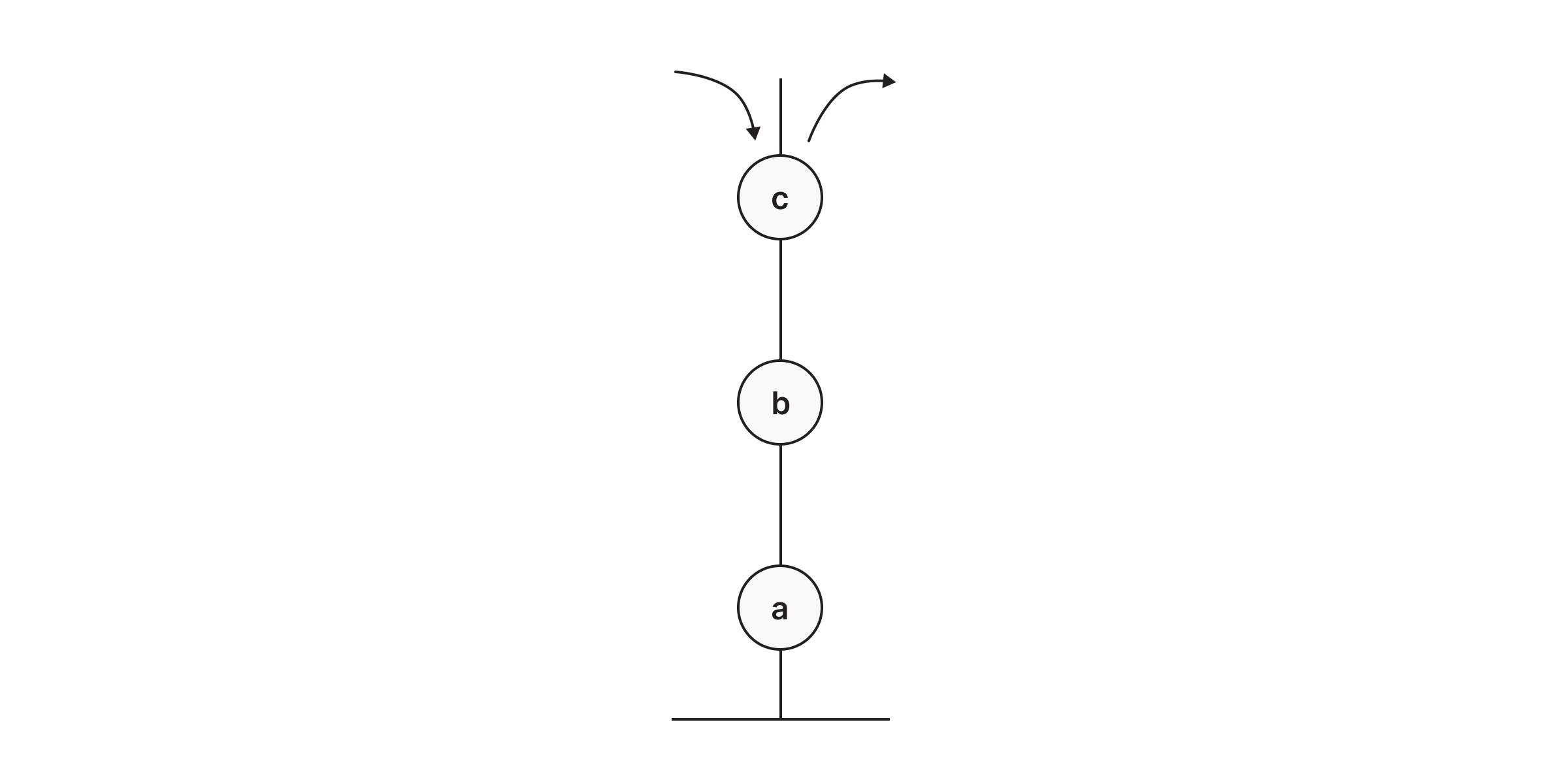
Stack is a linear data structure that follows a particular order in which the operations are performed. The order may be LIFO (Last In First Out) or FILO (First In Last Out). LIFO implies that the element that is inserted last, comes out first and FILO implies that the element that is inserted first, comes out last.

Representing a Stack in Memgraph

In Memgraph, we can represent a stack similar to how we represented a queue. The following query creates nodes and relationship :ON_TOPcode> between them, indicating that node A came first to the stack, followed by nodes B and C. Since the stack behaves in First In Last Out order, we can retrieve only the node that came last, in our case the node C.

CREATE (n1:Node {name: 'A'}), (n2:Node {name: 'B'}), (n3:Node {name: 'C'}),
(n3)-[:ON_TOP]->(n2)-[:ON_TOP]->(n1)

Operations with Stack

If we want to find out which node is on top of the stack and remove it, similar to how the Pop() function behaves, we can do that with the following query:

MATCH (a)-[:ON_TOP]->(b)
WHERE NOT exists(()-[:ON_TOP]->(a))
DETACH DELETE a

The query first matches all of the nodes that are on top of any other node and filters the node by those who don’t have nodes on top of them, resulting in the node on top of the stack.

If we want to add a node to the stack, mimicking the Push() function, we can achieve that with the following query:

MATCH (a)-[:ON_TOP]->(b)
WHERE NOT exists(()-[:ON_TOP]->(a))
CREATE (n4:Node {name:'D'})-[:ON_TOP]->(a)

Similar to the previous query, we first retrieve the node on the top of the stack and then create another node connected to that one with the :ON_TOP relationship.

Tree structure

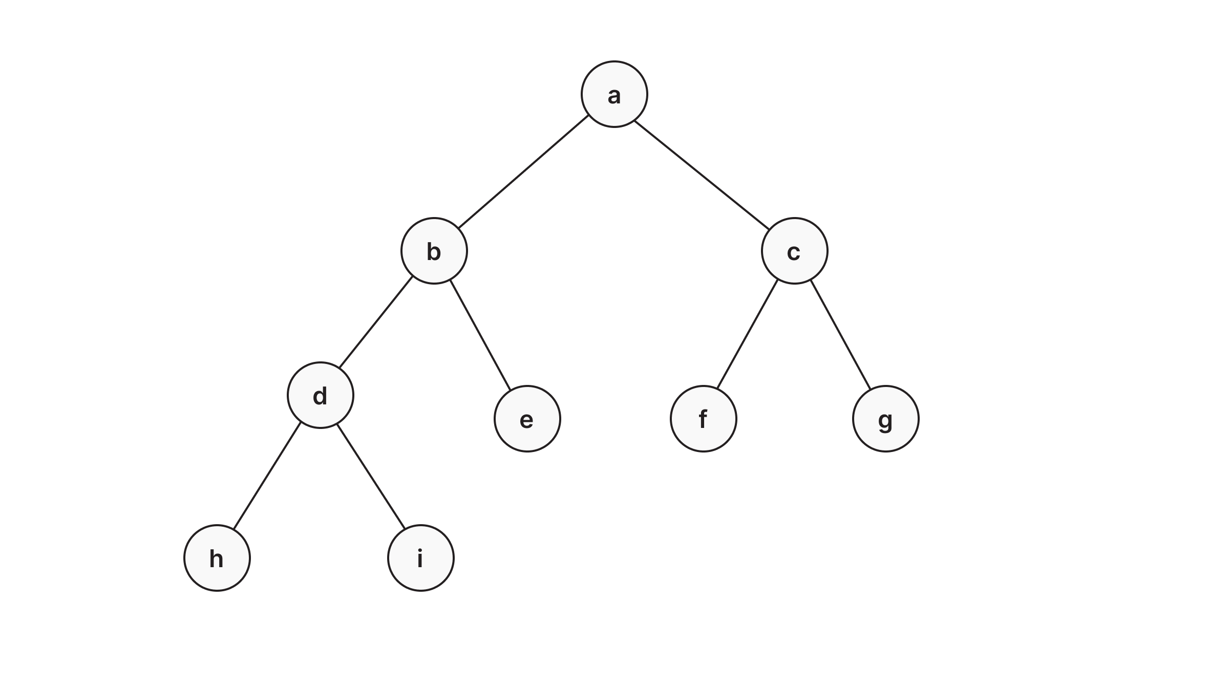
A tree organizes values hierarchically. Each entry in the tree is called a node and every node links to zero or more child nodes. Leaf nodes are nodes that are on the bottom of the tree (more formally: nodes that have no children). Each node in a tree has a depth: the number of links from the root to the node. A tree's height is the number of links from its root to the furthest leaf. (That's the same as the maximum node depth.)

How to represent Tree structure in Memgraph

Memgraph already has a structure similar to the tree, it has nodes connected with relationships, the only thing left to specify is the connection between those nodes, which node is the parent node and which is the child node.

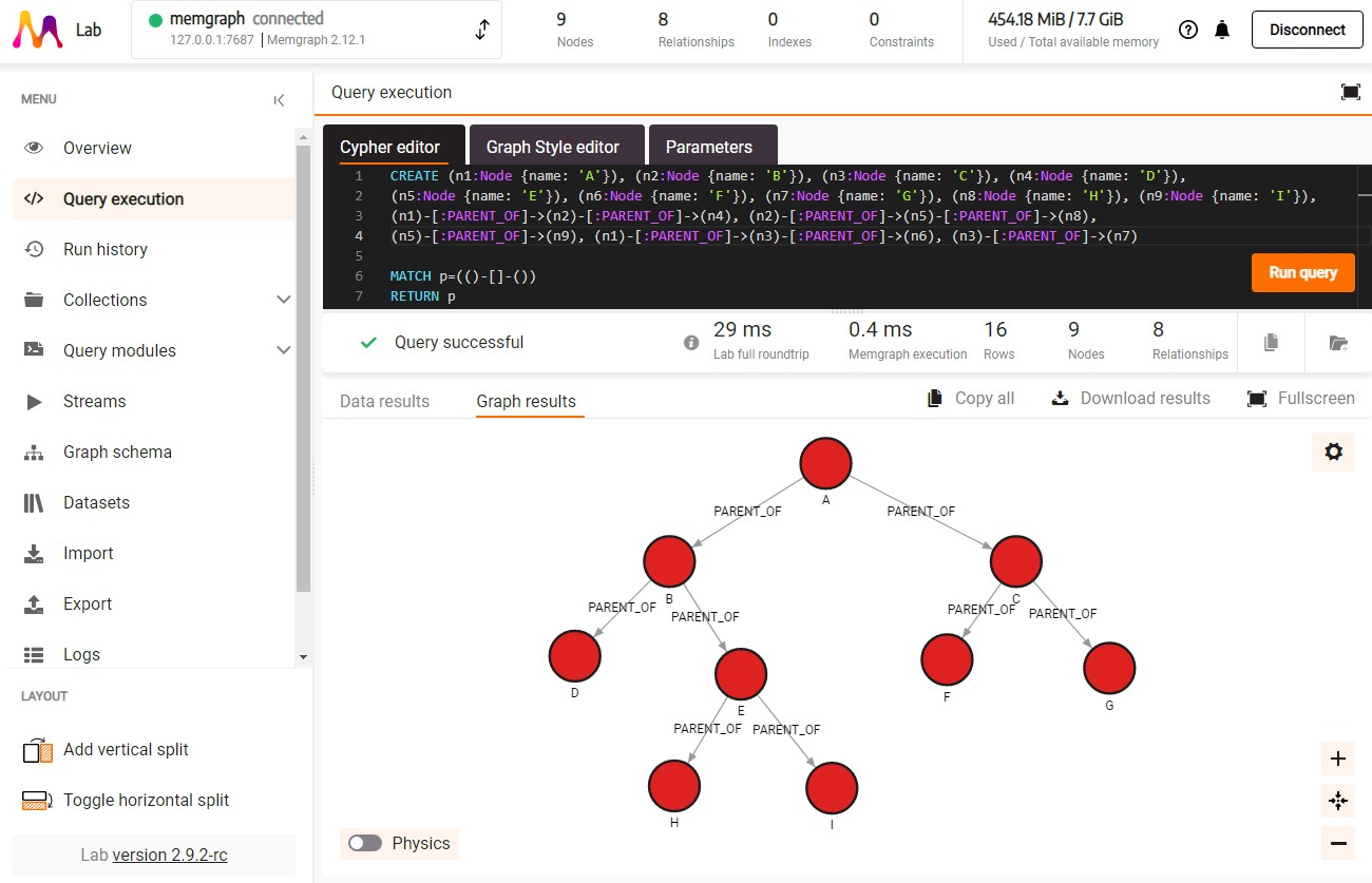
Let’s create a tree from the image above, the following query creates nodes named alphabetically from A to I with the relationship :PARENT_OF between them, indicating the connection.

CREATE (n1:Node {name: 'A'}), (n2:Node {name: 'B'}), (n3:Node {name: 'C'}), (n4:Node {name: 'D'}),
(n5:Node {name: 'E'}), (n6:Node {name: 'F'}), (n7:Node {name: 'G'}), (n8:Node {name: 'H'}), (n9:Node {name: 'I'}),
(n1)-[:PARENT_OF]->(n2)-[:PARENT_OF]->(n4), (n2)-[:PARENT_OF]->(n5)-[:PARENT_OF]->(n8),
(n5)-[:PARENT_OF]->(n9), (n1)-[:PARENT_OF]->(n3)-[:PARENT_OF]->(n6), (n3)-[:PARENT_OF]->(n7)

By running the following query, we’ll be able to visualize the newly created tree structure in Memgraph, shown in the image below.

MATCH p=(()-[]-()) RETURN p;

Traversing

In computer science, tree traversal (also known as tree search and walking the tree) is a form of graph traversal and refers to the process of visiting (e.g. retrieving, updating, or deleting) each node in a tree data structure, exactly once. Such traversals are classified by the order in which the nodes are visited. Here we'll mention two most popular algorithms for tree traversals, Breadth First Search and Depth First Search algorithms.

Breadth First Search (BFS) algorithm

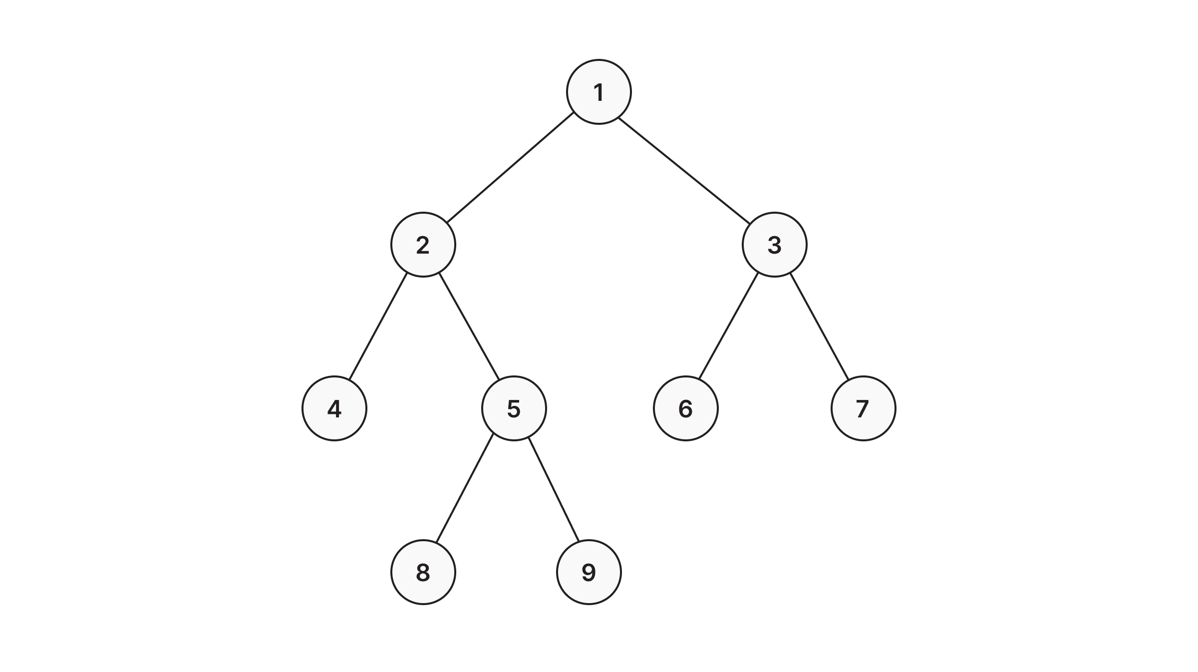
In breadth-first search (BFS) traversal starts from a single node, and the order of visited nodes is decided based on nodes' breadth (distance from the source node). This means that when a certain node is visited, it can be safely assumed that all nodes that are fewer relationships away from the source node have already been visited, resulting in the shortest path from the source node to the newly visited node.

Here's a sample tree, with the nodes labeled in the order they'd be visited in a BFS:

Running BFS in Memgraph

BFS in Memgraph has been implemented based on the relationship expansion syntax. There are a few benefits of the breadth-first expansion approach, instead of a specialized function. For one, it is possible to inject expressions that filter nodes and relationships along the path itself, not just the final destination node. Furthermore, it's possible to find multiple paths to multiple destination nodes. Also, it is possible to simply go through a node's neighborhood in a breadth-first manner.

The following query will show the shortest path between nodes A and H as a graph result:

MATCH path=(a {name: ‘A’})-[*BFS]->(h {name: ‘H’})
RETURN path;

To get the list of relationships, add a variable before the *BFS and return it as a result:

MATCH (a {name: ‘A’})-[relationships *BFS]->(h {name: ‘H’})
RETURN relationships;

Depth First Search (DFS) algorithm

Depth-first search (DFS) is an algorithm for traversing through the graph. The algorithm starts at the root node and explores each neighboring node as far as possible. The moment it reaches a dead-end, it backtracks until it finds a new, undiscovered node, then traverses from that node to find more undiscovered nodes. In that way, the algorithm visits each node in the graph.

Here's how a DFS would traverse the same example tree:

Running DFS in Memgraph

DFS in Memgraph has been implemented based on the relationship expansion syntax which allows it to find multiple relationships between two nodes if such exist. Below are several examples of how to use the DFS in Memgraph.

The following query will show all the paths from node A to node H:

MATCH path=(a {name: ‘A’})-[*]->(h {name: ‘H’})
RETURN path;

To get the list of all relationships, add a variable in the square brackets and return it as a result:

MATCH (a {name: ‘A’})-[relationships *]->(h {name: ‘H’})
RETURN relationships;

Takeaway

This article introduces data structures and their examples while covering the basics of graphs, demonstrating how data structures can be represented in Memgraph. If you have any remaining questions about data structures, their usage in Memgraph or Memgraph in general, feel free to join us on Discord and ask away!