Analyze Infrastructure Networks With Dynamic Betweenness Centrality

By Ante Pusic

11 min readApril 21, 2022

Remember when undersea internet cables came under attack by... sharks?!

In this blog post, you will explore how the loss of a connection can affect the global submarine internet cable network, and learn how to use dynamic betweenness centrality to efficiently analyze streamed data in Memgraph.

The loss of a cable is a textbook example of how a single change can immediately disrupt the entire network. To enable rapid response in such situations, our MAGE 🧙‍♂️ team has been adding online graph algorithms (Node2Vec, PageRank & community detection), whose magic ✨ is in updating previous outputs instead of computing everything anew.

Explore the Global Shipping Network

Prerequisites

In this tutorial, you will use Memgraph with:

Data

The dataset used in this blogpost represents the global network of submarine internet cables in the form of a graph whose nodes stand for landing points, the cables connecting them represented as relationships.

Landing points and cables have unique identifiers (id), and the landing points also have names (name).

A giant thank you to TeleGeography for sharing the dataset for their submarine cable map. ❤️

Exploration

Our Setup

With Docker installed, we will start Memgraph through it using the following command:

docker run -it -p 7687:7687 -p 3000:3000 memgraph/memgraph-platform

We will be working with Memgraph from a Jupyter notebook. To interact with Memgraph from there, we use GQLAlchemy.

Betweenness Centrality

Before we start exploring our graph, let’s quickly refresh that betweenness centrality of a node is the fraction of shortest paths between all pairs pairs of nodes in the graph that pass through it:

memgraph-betweenness-centrality

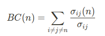
In the above expression, n is the node of interest, i, j are any two distinct nodes other than n, and σ_ij(n) is number of shortest paths from i to j (going through n).

The analysis of (internet) traffic flows, like what we are doing here, is an established use case for this metric.

Jupyter notebook

The Jupyter notebook is here – we can now go for a deep dive 🤿 in the data!

Preliminaries

First, let’s connect to our instance of Memgraph with GQLAlchemy and load the dataset.

from gqlalchemy import Memgraph

def load_dataset(path: str):
    with open(path, mode='r') as dataset:
        for statement in dataset:
            memgraph.execute(statement)

memgraph = Memgraph("127.0.0.1", 7687)    # connect to running instance
memgraph.drop_database()                  # make sure it’s empty
load_dataset('data/input.cyp')            # load dataset

Example

With everything set up, calling the betweenness_centrality_online module is a matter of a single Cypher query. As we are analyzing how changes affect the undersea internet cable network, we save the computed betweenness centrality scores for later.

memgraph.execute(
    """
    CALL betweenness_centrality_online.set()
    YIELD node, betweenness_centrality
    SET node.bc = betweenness_centrality;
    """
)

Let’s see which landing points have the highest betweenness centrality score in the network:

most_central = memgraph.execute_and_fetch(
    """
    MATCH (n: Node)
    RETURN n.id AS id, n.name AS name, n.bc AS bc_score
    ORDER BY bc_score DESC, name ASC
    LIMIT 5;
    """
)
for node in most_central:
    print(node)

{'id': 15, 'name': 'Tuas, Singapore', 'bc_score': 0.29099145440251273}
{'id': 16, 'name': 'Fortaleza, Brazil', 'bc_score': 0.13807572163430684}
{'id': 467, 'name': 'Toucheng, Taiwan', 'bc_score': 0.13361801370831092}
{'id': 62, 'name': 'Manado, Indonesia', 'bc_score': 0.12915295031722301}
{'id': 123, 'name': 'Balboa, Panama', 'bc_score': 0.12783714460527598}

Two of the above results, Singapore and Panama, have become international trade hubs owing to their favorable geographic position. They are highly influential nodes in other networks as well.

Dynamic Operation

This part brings us to MAGE’s newest algorithm – iCentral dynamic betweenness centrality by Fuad Jamour and others.^[1]. After each graph update, iCentral can be run to update previously computed values without having to process the entire graph, going hand in hand with Memgraph’s graph streaming capabilities.

You can set this up in Memgraph with triggers – pieces of Cypher code that run after database transactions.

memgraph.execute(
    """
    CREATE TRIGGER update_bc
    BEFORE COMMIT EXECUTE
        CALL betweenness_centrality_online.update(createdVertices, createdEdges, deletedVertices, deletedEdges)
        YIELD *;
    """
)

memgraph-shark-cuts-internet-cable

Let’s now see what happens when a shark (or something else) cuts off a submarine internet cable between Tuas in Singapore and Jeddah in Saudi Arabia.

memgraph.execute("""MATCH (n {name: "Tuas, Singapore"})-[e]-(m {name: "Jeddah, Saudi Arabia"}) DELETE e;""")

The above transaction activates the update_bc trigger, and previously computed betweenness centrality scores are updated using iCentral.

With the cable out of function, internet data must be transmitted over different routes. Some nodes in the network are bound to experience increased strain and internet speed might thus deteriorate. These nodes likely saw their betweenness centrality score increase. To inspect that, we’ll retrieve the new scores with betweenness_centrality_online.get() and compare them with the previously saved ones.

highest_deltas = memgraph.execute_and_fetch(
    """
    CALL betweenness_centrality_online.get()
    YIELD node, betweenness_centrality
    RETURN
        node.id AS id,
        node.name AS name,
        node.bc AS old_bc,
        betweenness_centrality AS bc,
        betweenness_centrality - node.bc AS delta
    ORDER BY abs(delta) DESC, name ASC
    LIMIT 5;
    """
)
for result in highest_deltas:
    print(result)
 
memgraph.execute("DROP TRIGGER update_bc;")

{'id': 111, 'name': 'Jeddah, Saudi Arabia', 'old_bc': 0.061933737931979434, 'bc': 0.004773934386713466, 'delta': -0.057159803545265966}
{'id': 352, 'name': 'Songkhla, Thailand', 'old_bc': 0.05259842296405675, 'bc': 0.07514804741735281, 'delta': 0.022549624453296065}
{'id': 15, 'name': 'Tuas, Singapore', 'old_bc': 0.29099145440251273, 'bc': 0.2730690696075149, 'delta': -0.017922384794997803}
{'id': 175, 'name': 'Yanbu, Saudi Arabia', 'old_bc': 0.0648358824682235, 'bc': 0.07561992914231867, 'delta': 0.010784046674095174}
{'id': 210, 'name': 'Dakar, Senegal', 'old_bc': 0.08708567541545133, 'bc': 0.09412362761485257, 'delta': 0.007037952199401246}

As seen above, the network landing point in Songkhla, Thailand had its score increase by 42.87% after the update. Conversely, other landing points became less connected to the rest of the network: the centrality of the Jeddah node in Saudi Arabia almost dropped to zero.

Performance

iCentral builds upon the Brandes algorithm^[2] and adds the following improvements in order to increase performance:

Process only the nodes whose betweenness centrality values change: after an update, betweenness centrality scores stay the same outside the affected biconnected component.
Avoid repeating shortest-path calculations: use prior output if it’s possible to tell it’s still valid; if new shortest paths are needed, update the prior ones instead of recomputing.
- Breadth-first search for computing graph dependencies does not need to be done out of nodes equidistant to both endpoints of the updated relationship.
- The BFS tree used for computing new graph dependencies (the contributions of a node to other nodes’ scores) can be determined from the tree obtained while computing old graph dependencies.

bcc_partition = memgraph.execute_and_fetch(
    """
    CALL biconnected_components.get()
    YIELD bcc_id, node_from, node_to
    RETURN
        bcc_id,
        node_from.id AS from_id,
        node_from.name AS from_name,
        node_to.id AS to_id,
        node_to.name AS to_name
    LIMIT 15;
    """
)
for relationship in bcc_partition:
    print(relationship)

Graphs of infrastructural networks, such as this one, fairly often consist of a number of smaller biconnected components (BCCs). As iCentral recognizes that betweenness centrality scores are unchanged outside the affected BCC, this can result in a significant speedup.

Algorithms: Online vs. Offline

An important property of algorithms is whether they are online or offline. Online algorithms can update their output as more data becomes available, whereas offline algorithms have to redo the entire computation.

The gold-standard offline algorithm for betweenness centrality is the one by Ulrik Brandes^[2]: it works by building a shortest path tree from each node of the graph and efficiently counting the shortest paths through dynamic programming.

In How to Identify Essential Proteins using Betweenness Centrality we built a web app to visualize protein-protein interaction networks with help of betweenness centrality.

However, we can easily see that updates often change only a tiny piece of the whole graph. Scalability means that one needs to take advantage of this by cutting down on repetition. To this end, we employed the fastest algorithm so far: iCentral. Let’s see how it stacks up against the Brandes algorithm in complexity.

Brandes: runs in O(|V||E|) time and uses O(|V| + |E|) space on a graph with |V| nodes and |E| relationships,
iCentral: runs in O(|Q||E_BC|) time and uses O(|V_BC| + |E_BC|) space. |V_BC| and |E_BC| are the counts of nodes and relationships in the affected portion of the graph; |Q| ≤ |V_BC| (see the Performance section for the |Q| set). NB: iCentral also saves time by avoiding repeated shortest-path calculations where possible; this varies by graph.

Another key trait of iCentral is that it can be run fully in parallel, just like the Brandes algorithm. With N parallel instances, this has the algorithm run N times faster, at the expense of requiring N times more space (each thread keeps a copy of the data structures).

Takeaways

Betweenness centrality is a very common graph analytics tool, but it is nevertheless challenging to scale up to dynamic graphs. To solve this, Memgraph has implemented the fastest yet online algorithm for it – iCentral; it joins our growing suite of streaming graph analytics.

Our R&D team is working hard on streaming graph ML and analytics. We’re happy to discuss it with you – ping us at Discord!

What’s Next?

It’s time to build with Memgraph! 🔨

Check out our MAGE open-source graph analytics suite and don’t hesitate to give a star ⭐ or contribute with new ideas. If you have any questions or you want to share your work with the rest of the community, join our Discord server.

References

[1] Jamour, F., Skiadopoulos, S., & Kalnis, P. (2017). Parallel algorithm for incremental betweenness centrality on large graphs. IEEE Transactions on Parallel and Distributed Systems, 29(3), 659-672.

[2] Brandes, U. (2001). A faster algorithm for betweenness centrality. Journal of Mathematical Sociology, 25(2), 163-177.