Optimizing Telco Networks With Graph Coloring & Memgraph MAGE

Introduction

It's lunchtime, you're hungry and can't wait for your food delivery to arrive. The courier is 10 minutes late, so you decide to give him a call to make sure he didn't get lost on his way. Unfortunately, every time you get hold of him, the call drops abruptly. Confused, you start wondering what's the problem.

Most likely, this is an issue on the network side due to something known as code assignment or code planning. This is a common optimization challenge in the telecommunication industry, which if done incorrectly causes errors when a phone is on the move.

In this tutorial, you will learn about the code assignment problem in telecommunication networks and how to solve it in a simple yet effective way using graph algorithms and Memgraph.

Understanding the Code Assignment in Telecommunication Networks

When making a call, the phone must have an established connection with the base station. The antenna on the base station has a particular signal strength that decreases with distance, so the phone should be connected to the base station nearby to provide the required quality. The major challenge is to ensure the quality of calls on the move. If the phone moves away from the base station, the signal diminishes, and the phone disconnects. To avoid call interruptions, the phone should find a new base station, the closest one at that moment, and connect to it.

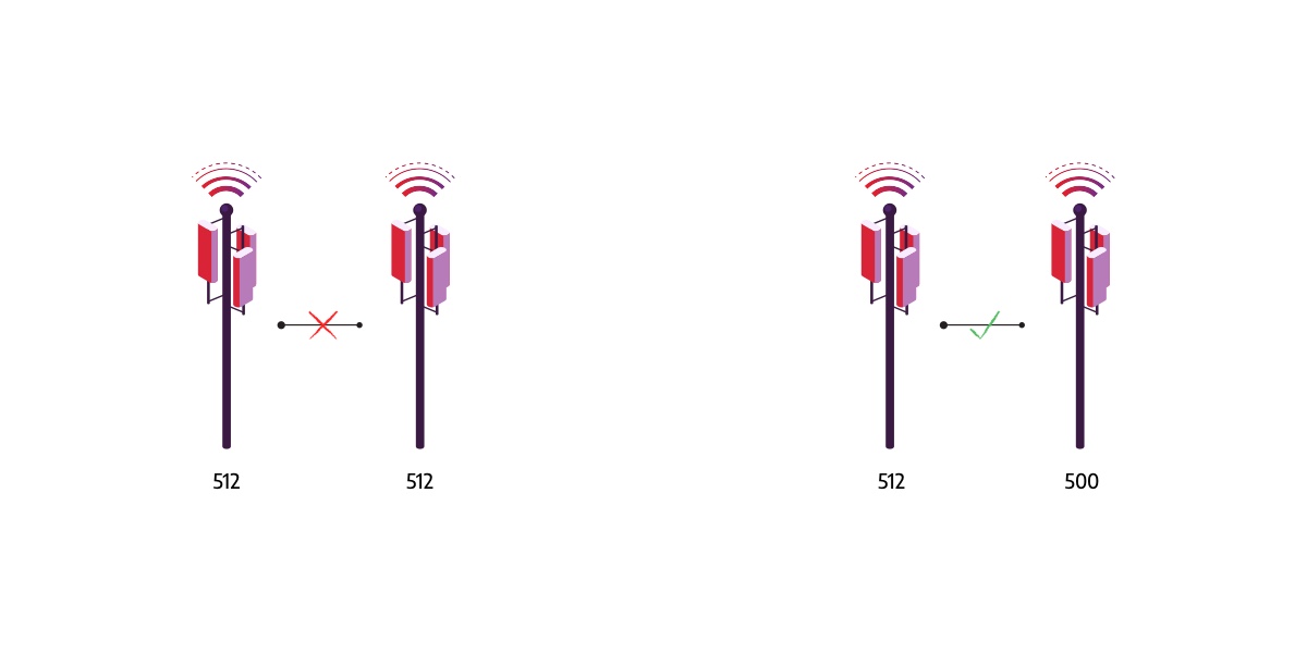
The phone needs to distinguish base stations to ensure a smooth transition between them. Various coding systems are used to identify base stations in the network. The number of different codes in a particular coding system is limited, so they need to be reused. However, if two close base stations have the same code their signals interfere and the phone cannot distinguish them. In case the phone moves between two base stations with the same code, the phone can incorrectly reconnect to the base station from which area it moves out, causing the call to drop.

Therefore, careful code assignment (code planning) is required to prevent neighboring base stations from using the same code. If done properly, code assigning significantly reduces the number of errors that occur while the phone switches base stations.

Modeling the Code Planning Problem with Graphs

The Telecommunications sector relies heavily on graphs, a mathematical structure used to represent a set of objects (called nodes or vertices), along with their relationships, also referred to as edges.

The graph model is a natural way to represent a telecommunication network, a group of communication devices and structure that supports the routing and transmission of information. Base stations and cell phones are part of that network. Naturally, nodes represent base stations, and edges connect those whose signals could interfere. These connections can contain additional information, a weight of an interference.

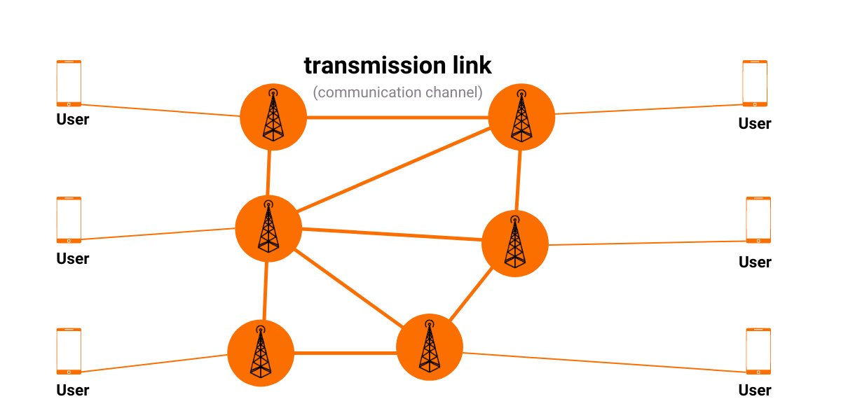
Code planning aims to assign codes and ensure that connected base stations are given different codes. In graph theory terminology, codes are equivalent to colors, and therefore code planning can be reformulated as graph coloring problem.

Graph coloring is the assignment of colors to nodes such that two nodes connected with an edge don't have the same color. The goal is to minimize the number of colors while correctly coloring a graph.

The graph coloring problem is a well-known NP-Hard problem, meaning that no time-efficient algorithm exists. It is practically impossible to find the minimal number of colors for graphs with over a hundred nodes. In a code planning scenario, we need to solve a slightly simpler problem. It is sufficient to find the k-coloring since the number of colors equals the number of available codes.

Prerequisites

To complete this tutorial, you will need either:

• Memgraph Platform: the complete streaming graph application platform that includes:
  • Memgraph DB - the database that holds your data
  • Memgraph Lab - an integrated development environment used to import data, develop, debug and profile database queries and visualize query results
  • mgconsole - command-line interface for running queries
  • MAGE - graph algorithms and modules library

or

• Memgraph Cloud: a hosted and fully-managed service that utilizes all Memgraph products such as MAGE and in-browser Memgraph Lab

Using the MAGE Graph Coloring Module

Memgraph introduces the concept of query modules, collections of user-written Cypher procedures intended to extend Cypher by implementing complex graph algorithms. Various query modules are already implemented and ready to use in an open-source project MAGE.

MAGE stands for Memgraph Advanced Graph Extensions. It is a project started by Memgraph to encourage developers to share innovative and useful query modules so the whole community can benefit from them.

Graph coloring is one of the algorithms included in MAGE. Algorithm implementation is inspired by Quantum Annealing, a simple metaheuristic frequently used for solving discrete optimization problems.

Building Your Graph Data Model

For this tutorial, you will be using an artificially generated dataset of base stations in Zagreb. It contains 200 nodes (Base Stations) and 2,388 edges (relations of type :CLOSE_TO ).

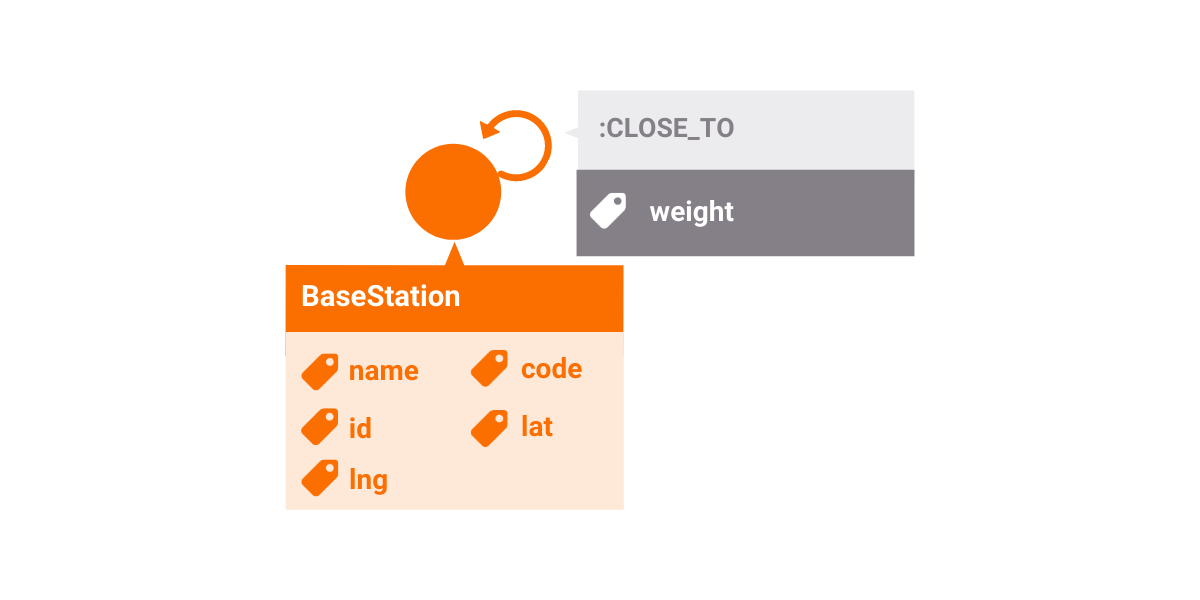
The essential properties of a node are lat, lng, and code. Properties lat and lng are abbreviations for latitude and longitude and represent coordinates of base stations on a map. The property code denotes the code assigned to the base station.

Two base stations are connected with an edge if they are close enough and strong enough for their signals to interfere. Since interference is symmetric (if the signals of the two base stations are in interference, then the first must interfere with the second and the second must interfere with the first), there is an edge for each direction. Every edge has a weight property that describes how strongly signals from base stations connected with this edge could interfere.

Importing the dataset

Once you connect to in-browser Memgraph Lab, either from Memgraph Cloud, or at localhost:3000 if you are using Memgraph Platform, navigate to the Datasets section in the sidebar and choose the dataset Base station network of Zagreb. The dataset will load automatically.

When the import is complete, you will be provided with a sample query that you can run to make sure everything works properly.

Now that your dataset is loaded, the next section will briefly describe how to visualize your data and call the graph coloring procedures. If you are already familiar with these concepts, skip to the section Developing a code planning solver.

Visualising the Graph With Memgraph Lab

Memgraph Lab is a simple yet powerful tool to help you visualize and explore your graph data.

When working with Geospatial data, Memgraph Lab automatically detects nodes that have numerical lat and lng properties to help you visualize your data points on a map without any additional effort.

Visualizing your data with Memgraph Lab is pretty easy. By running the following Cypher query, you should end up with results similar to the image below:

MATCH (n)-[e]-(m)
RETURN n, m, e;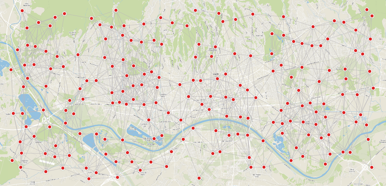

Executing the Graph Coloring Algorithm

Before writing and executing complex queries to solve the code planning task, we will outline the basic steps required to run the graph coloring procedure. You can find more details in the MAGE Spellbook.

The procedure can be invoked on the entire graph stored in Memgraph or on a selected subgraph. Moreover, you can use the default parameters or specify them arbitrarily to accommodate your data.

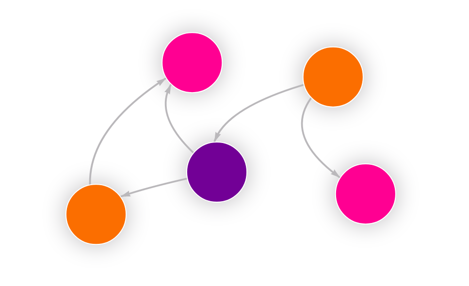
To get started, you will run a simple query that performs a fairly straightforward task. It calls the graph coloring procedure with default parameters and executes it on the whole graph.

CALL graph_coloring.color_graph() YIELD node, color;

What if you want to execute the algorithm on a subset of the graph?

In that case, it is necessary to first select the data, nodes and edges on which you want to perform the algorithm. To do that, you will need to use the MATCH clause, and your query will look something like this:

MATCH (a:BaseStation)-[e:CLOSE_TO]->(b:BaseStation)
WITH collect(a) AS nodes, collect (e) AS edges
CALL graph_coloring.color_subgraph(nodes, edges)
YIELD node, color
RETURN node, color;

The first part of the query matches two nodes with label BaseStation and the relationship between them with the label CLOSE_TO. The second part of the query, uses the WITH clause to combine the matching part of the query with the procedure call. Then, collected nodes and edges are stored in variables. Finally, you can call the procedure executing the algorithm on the subgraph passing nodes and edges as arguments.

If you are interested in running the graph coloring algorithm on custom data, you should tune the parameters to get the best possible results. Parameters are specified as named parameters in the dictionary passed to the procedure as an optional argument. You can consult the documentation to find out how a particular parameter affects the algorithm execution. For example, if you want to specify the number of colors, you can do it like this:

CALL graph_coloring.color_graph({no_of_colors: 3})
YIELD node, color
RETURN node, color;

If you run this query on the dataset used for this tutorial, you should get the following results:

Developing a Code Planning Solver

The starting point in building the code planning solver is to perform the graph coloring algorithm to obtain the correct assignment of codes to base stations. After running the procedure, you should somehow save the results in the code property of a node. For some applications, that may be enough. But you would often like to interpret the obtained results and notice errors in them to take corrective actions. Therefore, you will store additional information about errors in an edge and highlight that information in the visualization.

The return value of the procedure is a map that contains the mapping of nodes (Base Stations) to colors (codes). It is challenging to analyze the results in that form, so you will visualize them on a map. You will use the Style Editor in Memgraph Lab and customize the graph display to make the information you are interested in much more noticeable.

Therefore, developing a code planning solver can be divided into two parts. Finding and storing codes, along with error calculation, is the first part. The second part is the visualization of the results.

Finding and Storing Codes and Errors

Now that you have a basic understanding of utilizing graph coloring procedures, this part can be easily solved with the following query:

MATCH ()-[e :CLOSE_TO]->()
SET e.conflict = FALSE;
 
CALL graph_coloring.color_graph({num_of_colors : 10})
YIELD node, color
MATCH (n:BaseStation)
WHERE toString(id(n)) = node
SET n.code = toInteger(color);
 
MATCH (n:BaseStation)-[e:CLOSE_TO]->(m:BaseStation)
WHERE n.code = m.code
SET e.conflict = TRUE;
 
MATCH (n:BaseStation)-[e:CLOSE_TO]->(m:BaseStation)
RETURN n, m, e;

You should end up with the results shown below, and a simple visualization identical to the one in the data visualization section.

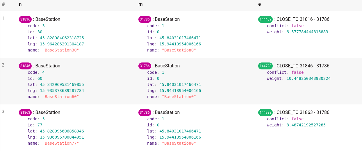
In the first part of the query, for each edge of type CLOSE_TO, you add a new property conflict with the initial value set to FALSE. The new property indicates whether the edge is conflicting - the edge connects base stations with the same code. Once you assign the codes, you will set the value of that property correctly. You will use these set values to highlight conflicting edges.

The second part of the query is calling the color_graph procedure from the graph_coloring module. The result of that part is the mapping of nodes identifiers to colors. You will store the results by finding nodes with the specified identifier and setting their property code to the assigned color.

In the third part of the query, you set the property conflict to TRUE for edges that connect the base stations with the same code. These edges are critical places in the network.

And finally, in the fourth part, you retrieve your graph.

Visualizing Your Results

Once the data is ready, it's time to style the display!

You will use the @NodeStyle directive for defining the style properties of a graph node. The directive is applied only to nodes with the label BaseStation. You can change the size of a node and border width. Also, you can add a little bit of a shadow by setting the shadow-size. To make the nodes look nicer, you can place images of base stations inside the nodes by setting the image-url field.

To make exploring the results easier, you will set the color of a node, border color, and shadow color based on the assigned codes.

Before all else, you need to know the maximum value of all possible codes. In the first line of the script, you use the built-in Define function to bind the maximum value of a code to the name max_code. If you use a different number of possible codes, change that value.

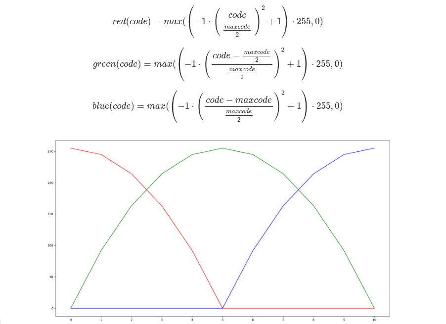
You will determine the color by setting the red, green, and blue components to the value given by the following functions. The function that describes the red component is defined to reach the maximum value when the code is equal to zero. The green component achieves a maximum for the code in the middle range of the allowed codes. The blue component function has a maximum for the largest possible code. The described functions are shown in the following image. The maximum code value in this example is 10.

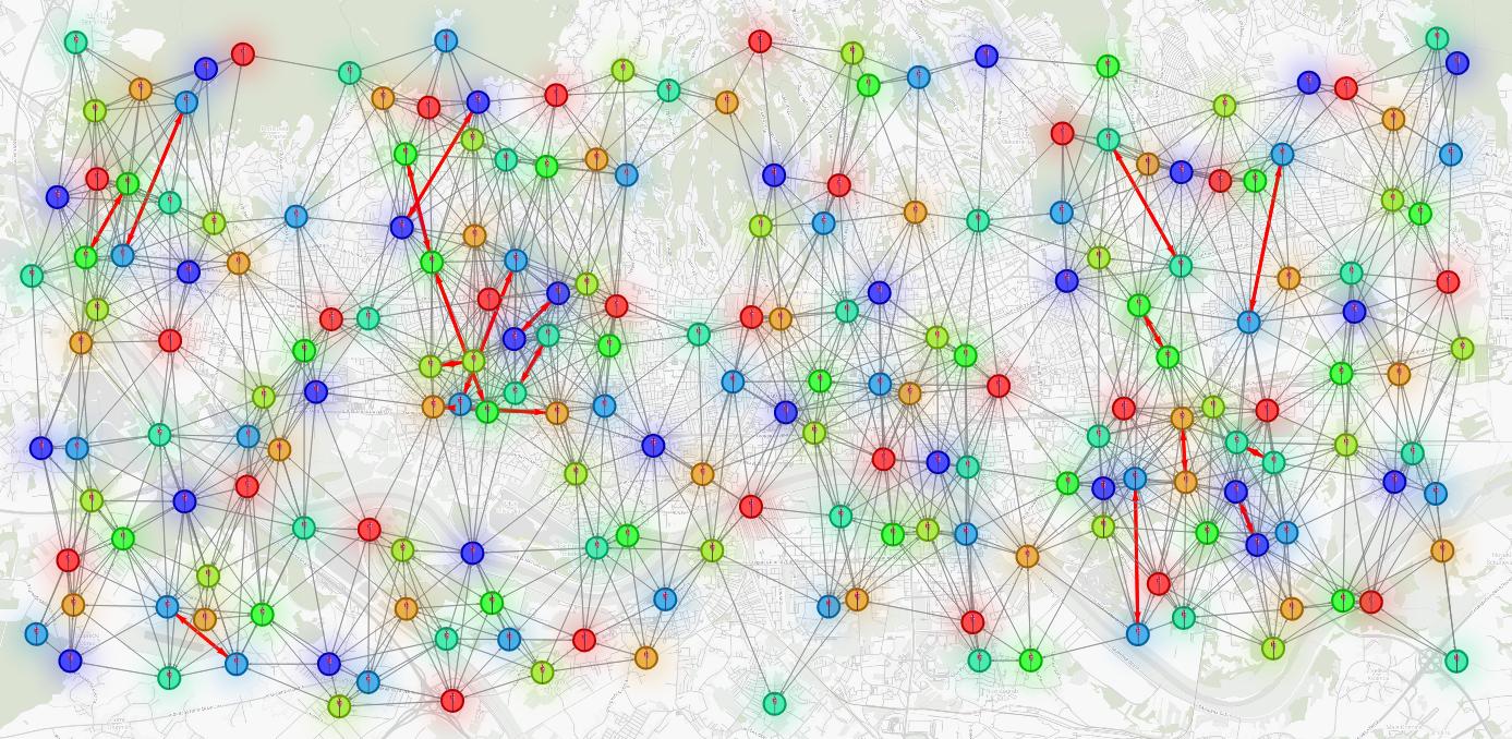
Lastly, you will make conflicting edges pop out by coloring them in red and setting their size to 15.

To achieve the described visualization, you will use a simple styling script. Just navigate to the style editor in Memgraph Lab (little gear icon in the right upper corner) and copy the following code. For a better understanding of the script, you can look at the Style script reference guide.

If you want to write and apply your style script, you can learn more about the style editor in the tutorial.

Define(max_code, 9)
Define(positive, Function(x, If(Less(x, 0), 0, x)))

@NodeStyle HasLabel(node, "BaseStation") {
  size: 50
  border-width: 2
  shadow-size: 30

  image-url: "https://i.imgur.com/4uxw9dD.png"

  color: Lighter(RGB(
    positive(Mul(Add(Mul(-1, Mul( Div(Add (Property(node, "code"), 0), Div(max_code,2) ) , Div(Add (Property(node, "code"), 0), Div(max_code,2) ) ) ), 1),255)),
    positive(Mul(Add(Mul(-1, Mul( Div(Add (Property(node, "code"), Mul(-1, Div(max_code,2))), Div(max_code,2) ) , Div(Add (Property(node, "code"), Mul(-1, Div(max_code,2))), Div(max_code,2) ) ) ), 1),255)),
    positive(Mul(Add(Mul(-1, Mul( Div(Add (Property(node, "code"), Mul(-1, max_code)), Div(max_code,2) ) , Div(Add (Property(node, "code"), Mul(-1, max_code)), Div(max_code,2) ) ) ), 1),255))
  ))

  border-color: Darker(RGB(
    positive(Mul(Add(Mul(-1, Mul( Div(Add (Property(node, "code"), 0), Div(max_code,2) ) , Div(Add (Property(node, "code"), 0), Div(max_code,2) ) ) ), 1),255)),
    positive(Mul(Add(Mul(-1, Mul( Div(Add (Property(node, "code"), Mul(-1, Div(max_code,2))), Div(max_code,2) ) , Div(Add (Property(node, "code"), Mul(-1, Div(max_code,2))), Div(max_code,2) ) ) ), 1),255)),
    positive(Mul(Add(Mul(-1, Mul( Div(Add (Property(node, "code"), Mul(-1, max_code)), Div(max_code,2) ) , Div(Add (Property(node, "code"), Mul(-1, max_code)), Div(max_code,2) ) ) ), 1),255))
  ))

  shadow-color: RGB(
    positive(Mul(Add(Mul(-1, Mul( Div(Add (Property(node, "code"), 0), Div(max_code,2) ) , Div(Add (Property(node, "code"), 0), Div(max_code,2) ) ) ), 1),255)),
    positive(Mul(Add(Mul(-1, Mul( Div(Add (Property(node, "code"), Mul(-1, Div(max_code,2))), Div(max_code,2) ) , Div(Add (Property(node, "code"), Mul(-1, Div(max_code,2))), Div(max_code,2) ) ) ), 1),255)),
    positive(Mul(Add(Mul(-1, Mul( Div(Add (Property(node, "code"), Mul(-1, max_code)), Div(max_code,2) ) , Div(Add (Property(node, "code"), Mul(-1, max_code)), Div(max_code,2) ) ) ), 1),255))
  )
}

@NodeStyle HasProperty(node, "name") {
  label: AsText(Property(node, "name"))
}

@EdgeStyle {
  width: If(And(HasProperty(edge, "conflict"), Property(edge, "conflict")),
            15,
            3)
  color: If(And(HasProperty(edge, "conflict"), Property(edge, "conflict")),
            red,
            grey)
}

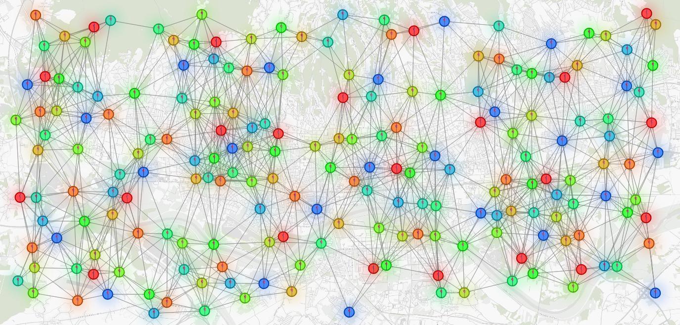
Congratulations, you now have a code planning solver! If everything works properly, you should get a visualization like the one below.

Exploring the Results

Aside from creating a beautiful visual representation, the applied style script helps you explore the data as well.

It is perfectly normal that despite running the sophisticated algorithms there are errors in results. There are several reasons why this can happen.

Sometimes it's impossible to correctly color the graph in the given number of colors due to the structure of the graph. For example, if we are asked to color three nodes that are all connected with an edge, no matter how hard you try, you cannot color them correctly in just two colors.

Another reason is that you use heuristics to solve graph coloring and they don't guarantee finding the perfect solution.

Finally, the reason could be that the algorithm's parameters were inadequately set. Whatever the reason, we want to be aware of places where the error occurred.

Let's take the first scenario and simulate a situation where errors occur due to an insufficient number of colors. To do this, you can run the following query:

MATCH ()-[e :CLOSE_TO]->()
SET e.conflict = FALSE;
 
CALL graph_coloring.color_graph({no_of_colors : 7})
YIELD node, color
MATCH (n:BaseStation)
WHERE toString(id(n)) = node
SET n.code = toInteger(color);
 
MATCH (n:BaseStation)-[e:CLOSE_TO]->(m:BaseStation)
WHERE n.code = m.code
SET e.conflict = TRUE;
 
MATCH (n:BaseStation)-[e:CLOSE_TO]->(m:BaseStation)
RETURN n, m, e;

You should end up with a few red edges. Base stations connected by red edges are close and have the same color. Those edges indicate places where base station signals interfere.

Bonus: Understanding Quantum Annealing

Quantum annealing (QA) is a metaheuristic developed based on ideas from physics.

A metaheuristic is an optimization approach that finds an approximate solution to a computationally expensive optimization problem.

An optimization is a process of finding the best value in the set of possible values, taking into account some criterion. Unlike exact algorithms, metaheuristics explore only a part of the whole solution space (set of all possible solutions).

While not performing the complete search can sometimes lead to not finding the perfect solution, this tradeoff is the main reason why heuristics are fast enough to be used in practice. In real-world cases, where it is important to find a "sufficiently good" solution in a short amount of time, a heuristic approach is the most efficient way to solve an optimization problem.

How Does Quantum Annealing Work?

QA is a simple strategy for exploring a solution space. The main idea is to start a search with several possible solutions. These solutions change through iterations and produce new "better" solutions. Each solution has a particular error value which depends on the error function that the algorithm optimizes. In the graph coloring scenario, the error function is often defined as the number of edges connecting nodes with the same color.

The algorithm is iterative. It applies several simple rules to change solutions in a loop (the same rules are applied multiple times). The algorithm terminates when a stop criterion is met, usually when the error becomes zero. One of the rules could be to randomly select the node involved in a conflict and change its colors.

Changes made in one iteration may not be permanent if they don't improve the solution. But, with a certain probability, the new solution is accepted even if its error is not reduced. In that way, the algorithm is prevented from converging to local minimums too early.

Conclusion

In this tutorial, you learned about the code assignment problem in telecommunication networks and built a simple yet effective solver for it using graph algorithms, Memgraph, and MAGE.

You learned how to execute and adjust the Graph Coloring algorithm, and how to visualize your results in Memgraph Lab.

MAGE is a versatile open-source library containing standard graph algorithms that you can run as Cypher procedures. While there are a lot of graph libraries out there which are great to perform graph computations, using MAGE and Memgraph provides you with additional benefits like persistent data storage and additional graph analytics capabilities. If your project requires a graph database, along with efficiently implemented graph algorithms, you should consider using Memgraph and MAGE .

If you found this tutorial interesting, you should try out the other algorithms part of the MAGE library.

Finally, if you are working on your own query module and would like to share it with other developers, take a look at the contributing guidelines. We would be more than happy to provide feedback and add the module to the MAGE repository.