Modeling, Visualizing, and Navigating a Transportation Network with Memgraph

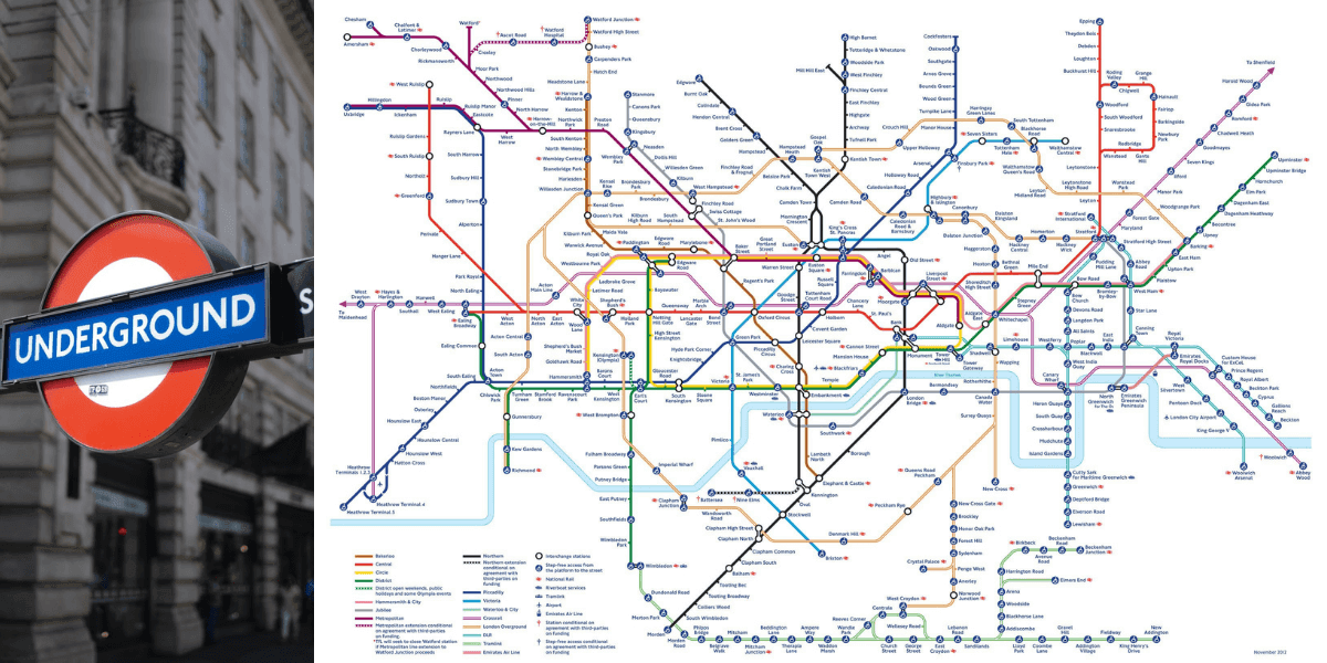
If riding a bike or walking is not an option, using public transport is the most eco-friendly way to travel around a city. Navigating a public transportation system can be confusing and complicated.

As a passenger, you usually want to know how to get from one station to another and where to change lines to make your journey as optimal as possible. In essence, the problem is finding the shortest path in the complex network of stations and lines. This type of problem is a typical graph use-case. Graphs are used for modeling and navigating complex network problems across a variety of domains including transportation, cybersecurity, fraud detection, and many more.

In this tutorial, you will explore how to use graphs to model, visualize, and navigate a transportation network. You will learn how to import the London Tube dataset into Memgraph and visualize it on a map using Memgraph Lab. Next, you will learn how to use the Cypher query language and graph algorithms to help you explore the London Tube network and find your way around the city without getting lost or wasting hours being stuck in traffic.

Prerequisites

To complete this tutorial, you will need:

• An installation of Memgraph DB: a native, in-memory graph database. To install Memgraph DB and set it up, please follow the Docker Installation instructions on the Installation guide.
• An installation of Memgraph Lab: an integrated development environment used to import data, develop, debug and profile database queries and visualize query results.
• The London Tube network dataset which you can download here.

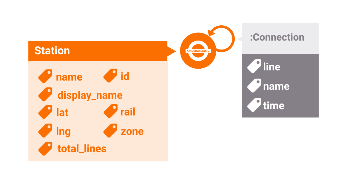
Defining the Graph Data Model

For this tutorial, you will be using the London Tube network dataset published by Nicola Greco. It contains 302 Stations (nodes) and 812 Connection (edges). The node lat and lng properties represent the coordinates of a station and will also be important to visualize the data on a map.

Two stations are connected with an edge of the type :Connection if they are adjacent. Since trains travel both ways, there is an edge for each direction.

Every edge has a time property that represents the time (in minutes) needed to travel between two stations and a line property which will make more sense after you add a name property later in this tutorial.

Now that you have defined your schema, you're ready to import your dataset.

Importing the Dataset using the CVS Import Tool

The first step is loading data into Memgraph. Memgraph comes with tools for importing data into the database. For this tutorial, you will be using the CSV Import Tool.

The CSV import tool should be used for the initial bulk ingestion of data into Memgraph. Upon ingestion, the CSV importer creates a snapshot that will be used by the database to recover its state on the next startup. You can learn about snapshots here.

Formating the CSV File

Each row of a CSV file represents a single entry that should be imported into the database. Both nodes and relationships can be imported into the database using CSV files.

To get all relevant data you will need three files. The first one contains data about nodes (stations.csv), the other two contain data about relationships (connections.csv and connections-reverse.csv). Each CSV file must have a header that describes the data. stations.csv has the following header:

id:ID(STATION),lat:double,lng:double,name:string,display_name:string,zone:int,total_lines:int,rail:int

The ID field type sets the internal ID that will be used for the node when creating relationships. It is optional and nodes that don't have an ID value specified will be imported, but can't be connected to any relationships.

When importing relationships, the START_ID field type sets the start node that should be connected with the relationship to the end node with END_ID. The field must be specified and the node ID must be one of the node IDs that were specified in the node CSV files.

The files connections.csv and connections-reverse.csv are identical except for the header. That’s because we need connections in both directions so, rather than creating missing relationships after importing the data, you can import the second file with a header where you switch START_ID and END_ID. As a result, you get a copy of every relationship from the first file, only in the opposite direction.

:END_ID(STATION),:START_ID(STATION),line:int,time:int

:START_ID(STATION),:END_ID(STATION),line:int,time:int

Using the CSV Import Tool

[NOTE] If your Memgraph database instance is running, you need to stop it before continuing to the next step.

First you need to copy the CSV files where the Docker image can see them. Navigate to the folder that contains the data files and run the following commands:

docker container create --name mg_import_helper -v mg_import:/import-data busybox
docker cp connections.csv mg_import_helper:/import-data
docker cp connections-reverse.csv mg_import_helper:/import-data
docker cp stations.csv mg_import_helper:/import-data
docker rm mg_import_helper

The two main flags that are used to specify the input CSV files are --nodes and --relationships. Labels for nodes (Station) and type for relationships (:Connection) need to be set on import because the CSV files don’t contain this information.

You can run the importer with the following command:

docker run -v mg_lib:/var/lib/memgraph -v mg_etc:/etc/memgraph -v mg_import:/import-data /
    --entrypoint=mg_import_csv memgraph /
    --nodes Station=/import-data/stations.csv /
    --relationships Connection=/import-data/connections.csv --relationships Connection=/import-data/connections-reverse.csv /
    --data-directory /var/lib/memgraph true --storage-properties-on-edges true

You can now start Memgraph by running the following command:

docker run -v mg_lib:/var/lib/memgraph -p 7687:7687 memgraph:latest --data-directory /var/lib/memgraph

If you have additional questions about the CSV Import Tool, take a look at our documentation: CSV Import Tool.

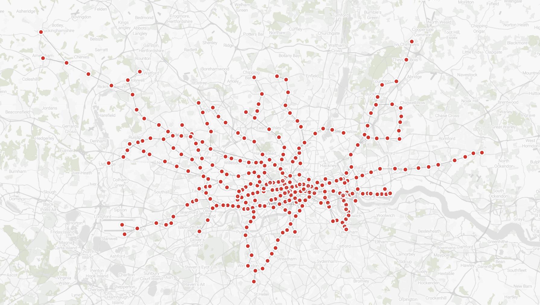
Visualising the Graph With Memgraph Lab

Once you have the data in Memgraph, visualizing it with Memgraph Lab is pretty easy. Memgraph Lab automatically detects nodes that have numerical lat and lng properties. To get your graph, run the following Cypher query:

MATCH (n)-[r]-(m)
RETURN n,r,m;

If everything works properly, you should get a visualization similar to the one below.

Adding a Property to the Edges

The line property doesn't make much sense because we usually recognize London Tube lines by their names or colors. The map will be more confusing than helpful unless you add a name property to the edges.

The following Cypher query uses the CASE expression which allows multiple predicates to be listed. The first one that evaluates to true is matched, and the result of the expression provided after the THEN keyword is used to set the value of the name property on a relationship.

MATCH (n)-[r]-(m)
SET r.name = CASE
WHEN r.line = 1  THEN "Bakerloo Line"
WHEN r.line = 2  THEN "Central Line"
WHEN r.line = 3  THEN "Circle Line"
WHEN r.line = 4  THEN "District Line"
WHEN r.line = 5  THEN "East London Line"
WHEN r.line = 6  THEN "Hammersmith & City Line"
WHEN r.line = 7  THEN "Jubilee Line"
WHEN r.line = 8  THEN "Metropolitan Line"
WHEN r.line = 9  THEN "Northern Line"
WHEN r.line = 10 THEN "Piccadilly Line"
WHEN r.line = 11 THEN "Victoria Line"
WHEN r.line = 12 THEN "Waterloo & City Line"
WHEN r.line = 13 THEN "Docklands Light Railway"
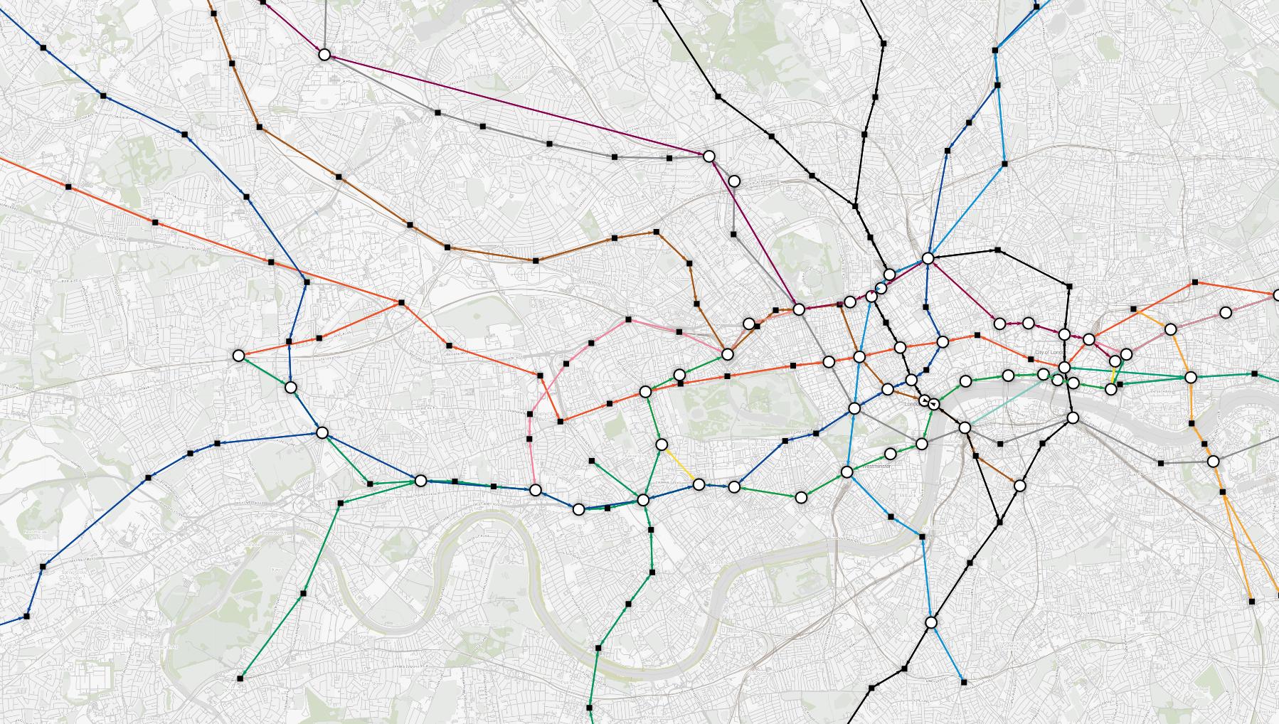
END;

Styling The Graph

While the dataset makes much more sense now, the styling of the map is still a bit too uniform. You can style the map to your liking by using the Style editor in Memgraph Lab. You can read more about the style editor in this tutorial.

First, let's make stations smaller and shaped like squares. A white circle with a black border is reserved for interchange stations (where you can switch between lines). To accomplish this, you will use the following styling script:

@NodeStyle HasLabel(node, "Station") {
    size: 15
    color: black
    shape: "square"
    color-hover: red
    color-selected: Darker(red)
}

@NodeStyle Greater(Property(node, "total_lines"), 1) {
    size: 30
    shape: "dot"
    border-width: 2
    border-color: black
    color: white
    color-hover: red
    color-selected: Darker(red)
}

@NodeStyle HasProperty(node, "name") {
    label: AsText(Property(node, "name"))
}

Now you can add the most important thing, the iconic line colors! To do this, you will use the following script:

@EdgeStyle HasProperty(edge, "name") {
  label: AsText(Property(edge, "name"))
  width: 10
}

@EdgeStyle Equals(Property(edge, "line"),1)  {color: #AE6017}
@EdgeStyle Equals(Property(edge, "line"),2)  {color: #F15B2E}
@EdgeStyle Equals(Property(edge, "line"),3)  {color: #FFE02B}
@EdgeStyle Equals(Property(edge, "line"),4)  {color: #00A166}
@EdgeStyle Equals(Property(edge, "line"),5)  {color: #FBAE34}
@EdgeStyle Equals(Property(edge, "line"),6)  {color: #F491A8}
@EdgeStyle Equals(Property(edge, "line"),7)  {color: #949699}
@EdgeStyle Equals(Property(edge, "line"),8)  {color: #91005A}
@EdgeStyle Equals(Property(edge, "line"),9)  {color: #000000}
@EdgeStyle Equals(Property(edge, "line"),10) {color: #094FA3}
@EdgeStyle Equals(Property(edge, "line"),11) {color: #0A9CDA}
@EdgeStyle Equals(Property(edge, "line"),12) {color: #88D0C4}
@EdgeStyle Equals(Property(edge, "line"),13) {color: #00A77E}

Your graph should now look like this:

Exploring the Graph Network

Now that you have your graph data loaded into Memgraph and visualizations set up in Memgraph Lab, you are ready to start exploring the London Tube network by using graph traversals and algorithms.

Let's say you're planning a trip and want to find a hotel near a well-connected station.

By using the following Cypher query, you will find which stations have the most connections to other stations:

MATCH (s1:Station)-[:Connection]->(s2:Station)
WITH DISTINCT s2.name as adjacent, s1.name as name
RETURN name AS Station_name, COUNT(adjacent) AS Total_connections
ORDER BY Total_connections DESC LIMIT 10;

For every station, the first part of the query matches all stations that are one degree apart. The second part counts connections and returns a list of the 10 most connected stations.

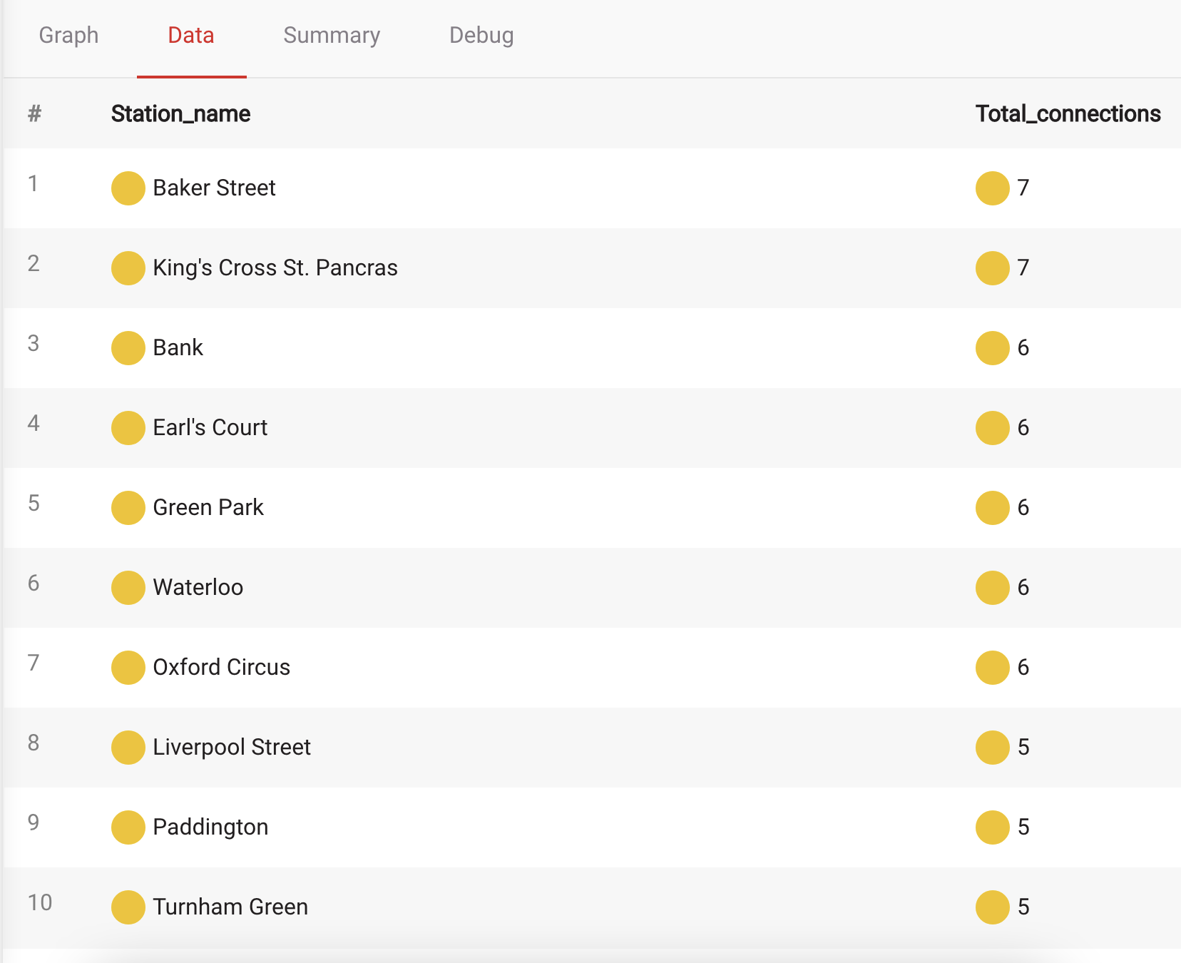
Now that you have your list, King's Cross St. Pancras is the obvious choice. You can easily check what Tube lines you can access from King's Cross St. Pancras by running the following query:

MATCH (:Station {name:"King's Cross St. Pancras"})-[r]-(:Station)
WITH DISTINCT r.name AS line
RETURN line;

Let's say you're traveling on a budget and you want to stay in the first fare zone to keep your transportation cost low. In this case, you can use the Breadth-First algorithm to find out what stations you can get to from St. Pancras while staying in the first fare zone:

MATCH p = (s1:Station {name:"King's Cross St. Pancras"})
          -[:Connection * bfs (e, n | n.zone = 1)]-
          (s2:Station)
UNWIND (nodes(p)) as rows
WITH DISTINCT rows.name as Station
RETURN Station LIMIT 10;

(e, n | n.zone = 1) is called a filter lambda. It's a function that takes an edge symbol e and a node symbol n and decides whether this edge and node pair should be considered valid in breadth-first expansion by returning true or false. In this example, the lambda is returning true if station is in the first fare zone.

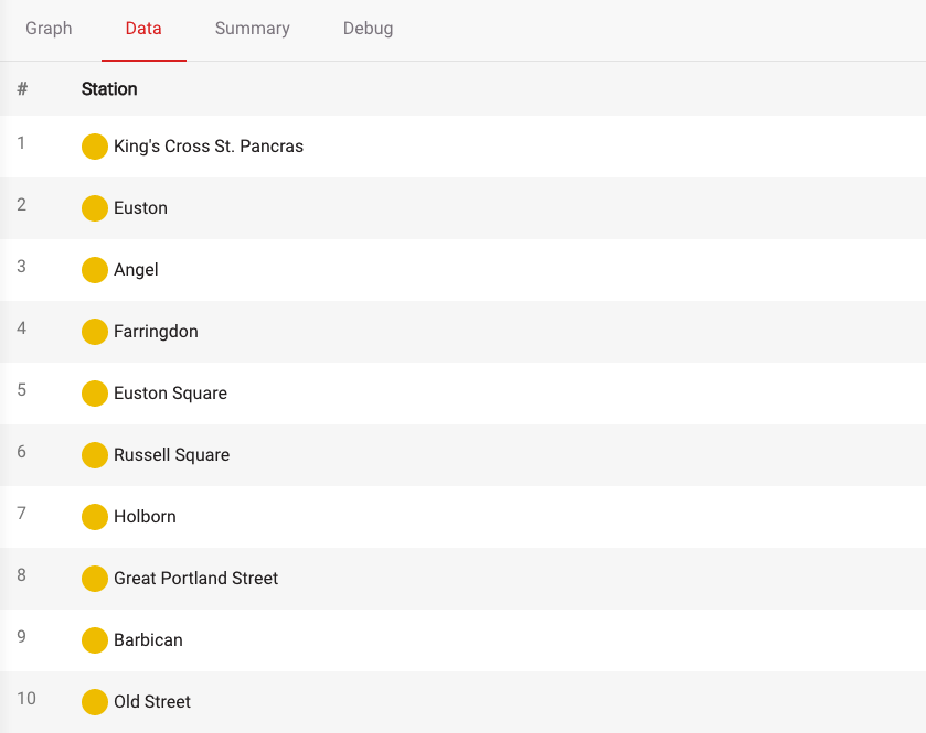
Or if you are more of a visual person, you can visualize your results by running the following query:

MATCH p = (:Station {name:"King's Cross St. Pancras"})
          -[:Connection * bfs (e, n | n.zone = 1)]-
          (:Station)
RETURN p;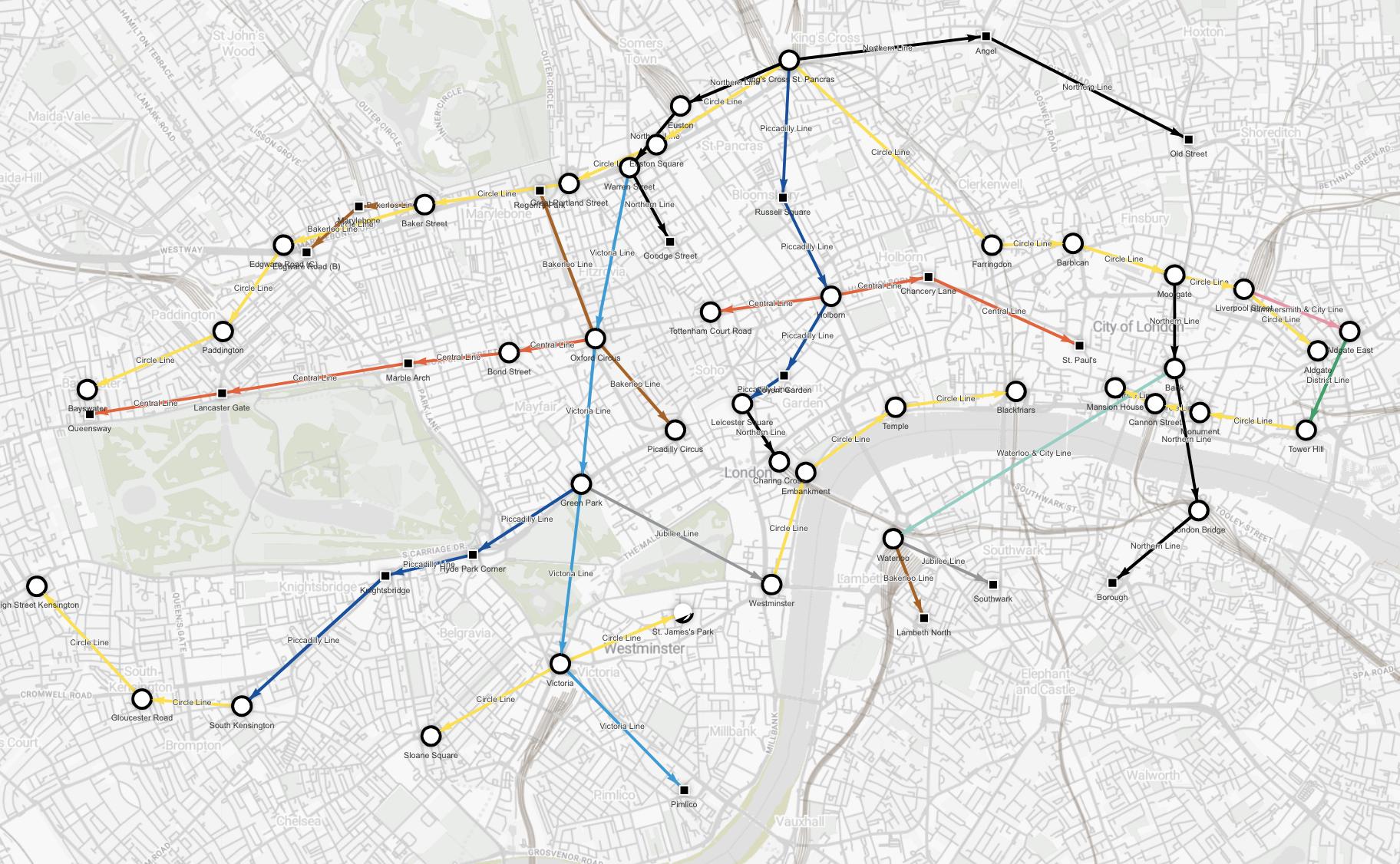

Let's say you have just arrived at London Heathrow airport. You are probably tired and in desperate need of a shower and nap but you'd love to stop by Big Ben, which is located at the Westminster tube station, on your way to your hotel.

Lucky for you, Memgraph can help you find the quickest route in no time!

Pathfinding algorithms are one of the classical graph problems and have been researched since the 19th century. The Shortest Path algorithm calculates a path between two nodes in a graph such that the total sum of the edge weights is minimized. The syntax here is similar to breadth-first search syntax. Instead of a filter lambda, we need to provide a weight lambda and the total weight symbol. Given an edge and node pair, weight lambda must return the cost (time) of expanding to the given node using the given edge.

MATCH p = (s1:Station {name: "Heathrow Terminal 4"})
          -[edge_list:Connection *wShortest (e, n | e.time) time]-
          (s2:Station {name: "Westminster"})
RETURN *;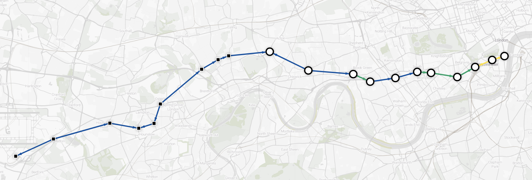

This route will get you from Heathrow to Westminster in 43 minutes, but there are delays on Circle and District lines, so you want exclude them from the search. You can combine weight and filter lambdas in the shortest-path query:

MATCH p = (s1:Station {name: "Heathrow Terminal 4"})
          -[edge_list:Connection *wShortest (e, n | e.time) time (e, n | e.name != "Circle Line" AND e.name != "District Line")]-
          (s2:Station {name: "Westminster"})
RETURN *;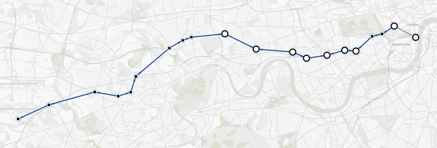

The new route is only 3 minutes longer, but you'll avoid delays.

And the shortest route from Westminster will get you to the hotel in 10 minutes (with Circle and District lines excluded).

MATCH p = (s1:Station {name: "Westminster"})
          -[edge_list:Connection *wShortest (e, n | e.time) time (e, n | e.name != "Circle Line" AND e.name != "District Line")]-
          (s2:Station {name: "King's Cross St. Pancras"})
RETURN *;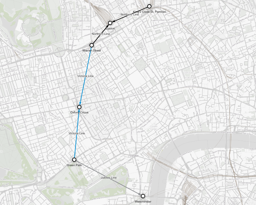

It is surprising how many of London’s museums and galleries are free to visit. The British Museum should definitely be your first choice! Although you can spend hours there, you want to see a little bit of everything so let's add a few more options.

Tottenham Court Road station is nearest to the British Museum and it will be your first stop. South Kensington station is within walking distance of three amazing museums: Science Museum, Natural History Museum, and Victoria and Albert Museum. To find the optimal route for your trip, you can use the following Cypher query:

MATCH p = (:Station {name: "King's Cross St. Pancras"})
          -[:Connection *wShortest (e, n | e.time) time1]-
          (:Station {name: "Tottenham Court Road"})
          -[:Connection *wShortest (e, n | e.time) time2]-
          (:Station {name: "South Kensington"})
RETURN p, time1 + time2 AS total_time;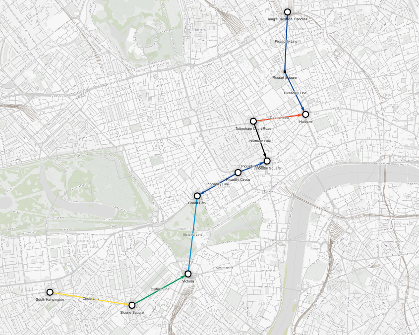

Conclusion

In this tutorial, you learned how to use Memgraph and Cypher to model and navigate a complex transportation network. With the help of graph algorithms, you found the optimal routes and learned how to visualize data using Memgraph Lab to get the most out of it. If you are interested in exploring another graph route planning tutorial, you can check out the Exploring the European Road Network demo on Memgraph Playground.

A friend once told me:

"You can never get lost in London, you just have to find a Tube station and you'll know where you are.”

I would say:

"You can never get lost in London, you just have to use Memgraph and find the shortest path!"

Remember, always stand on the right, and don’t forget to mind the gap!