
Building Skygraph: A Google Flights-like App with Memgraph and Cypher
Building Skygraph: A Google Flights-Like App Using Memgraph and Cypher
Remember the last time you booked a flight? You probably went to a search engine, typed in your departure and destination, and then spent a lot of time looking through endless lists of flights, trying to find the cheapest or fastest one. But what if you could do all of that with a single query?
In my recent seminar paper, "Skygraph: Find Your Ideal Vacation in Europe," I explored how graph databases can solve this problem. I built a Google Flights-like application called Skygraph, using Memgraph to model the complex web of European flight routes for a specific week in August.
In this article, I'll walk you through how I imported the data and, more importantly, how I used the power of the Cypher query language to quickly find the best flight options.
The Skygraph Data Model
To build a flight search engine, our model is composed of two types of nodes and two types of relationships.
We have City nodes, which have properties:
namepopulationcountry
I also included cities that do not have their own airports to allow for a more comprehensive search, enabling the application to find the nearest airport for any given city.
Airport nodes have properties:
code→ The unique IATA airport code, like ZAG for Zagrebcitycountry
These nodes are connected by two types of edges:
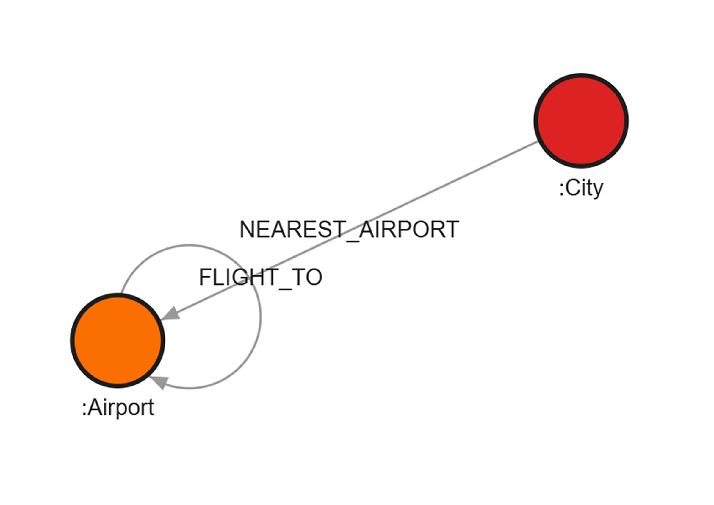
NEAREST_AIRPORT: Connects aCitynode to its closestAirportnode and has akmDistanceToNearestAirportproperty that stores the air distance in kilometers. This is a crucial link for translating a user's city search into a viable airport departure point.FLIGHT_TO: ConnectsAirportnodes and has the following properties that helps give us all the details we need to find the optimal flight path:company→ the airlinedepartureTimestamparrivalTimestamp→ Flight date and timedurationMinutes→ The flight duration in minutespriceEur→ The price in Euros
A visual representation of this schema can be seen in the diagram below:
Setting Up The Database In Memgraph
For installation and use, a variety of options are available. For this project, the 14-day free trial of Memgraph Cloud and the built-in Memgraph Lab UI were chosen, allowing work to be done directly from a web browser without any installation.
A good practice is to divide the data into separate CSV files for each node and edge type, which was followed here. 4 CSV files were prepared for this project:
nodesCities.csvnodesAirports.csvpathCityAirportDistance.csvpathsFlights.csv
Using the "CSV file import" option in the UI, the data for City and Airport nodes was first loaded from nodesCities.csv and nodesAirports.csv, respectively.
For these nodes, properties were defined, including setting Required and Unique properties such as the name for City nodes and code for Airport nodes. Indexes were not set, a common practice with graph databases on smaller datasets, as they are optimized for fast traversals.
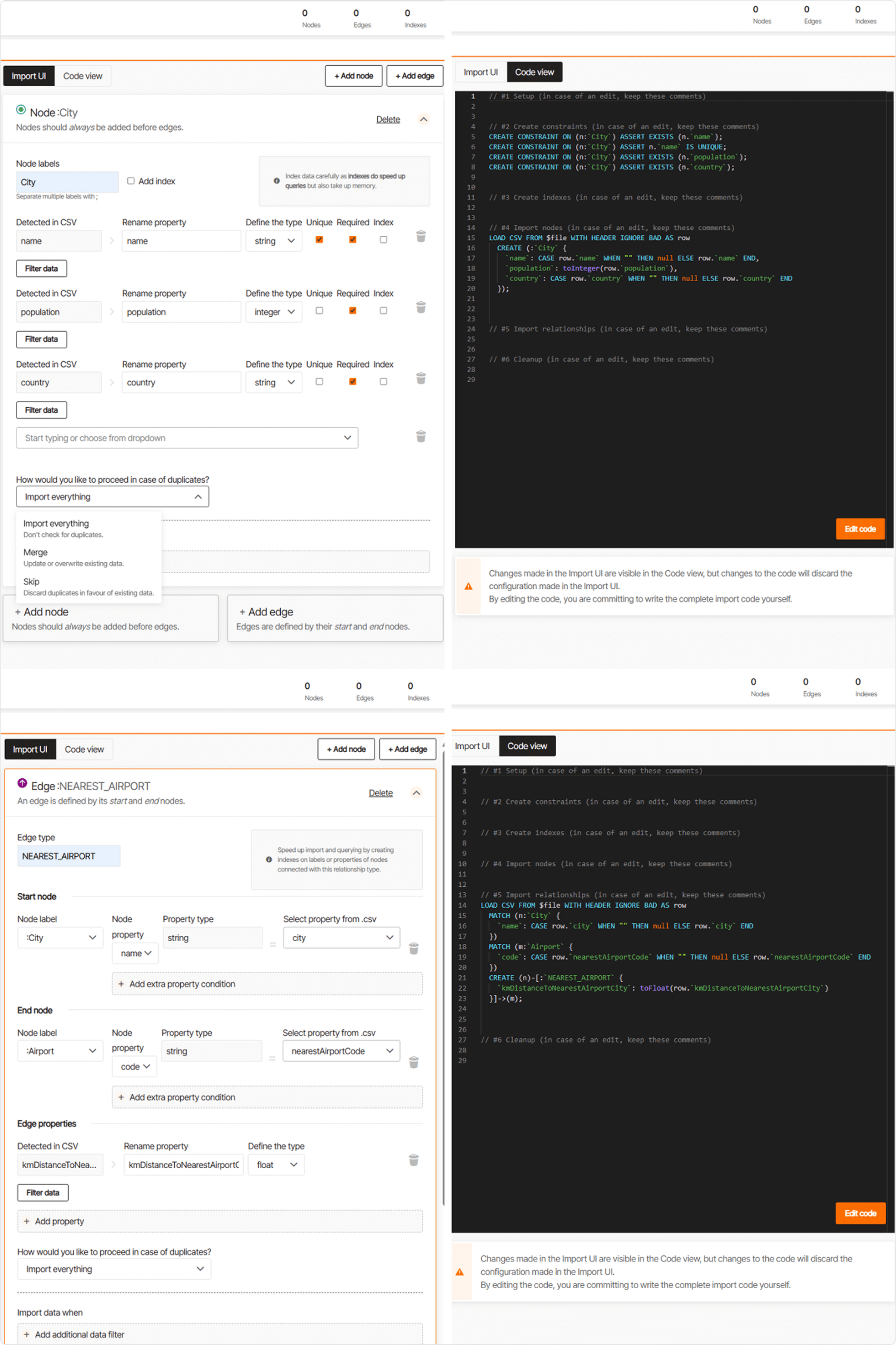
The NEAREST_AIRPORT edges were then imported from pathCityAirportDistance.csv. The UI for importing edges is a bit different from importing nodes, as it requires defining the start and end nodes of the relationship and connecting them by matching properties.
In this case, a City node's name property was matched to a corresponding city in the CSV, and an Airport node's code property was matched to the nearest airport code in the CSV. The process for importing nodes and edges is illustrated below:
The final step involved creating the FLIGHT_TO relationships. Since this required some custom data manipulation and filtering, the pathsFlights.csv file was loaded, and a custom Cypher query was written and executed.
LOAD CSV FROM $file WITH HEADER IGNORE BAD AS row
WITH
    row,
    row.departureAirport AS depCode,
    row.destinationAirport AS destCode
WHERE row.price IS NOT NULL AND row.price <> "Price unavailable"
MATCH (n:Airport { code: depCode })
MATCH (m:Airport { code: destCode })
CREATE (n)-[:FLIGHT_TO {
    company: row.company,
    departureTimestamp: localDateTime(row.departureTimestamp),
    arrivalTimestamp: localDateTime(row.arrivalTimestamp),
    durationMinutes: toInteger(row.duration),
    priceEur: toFloat(row.price)
}]->(m);
After all the data was successfully imported, the graph consisted of a total of 118 nodes and 45,517 edges.
Query Execution and Data Analysis
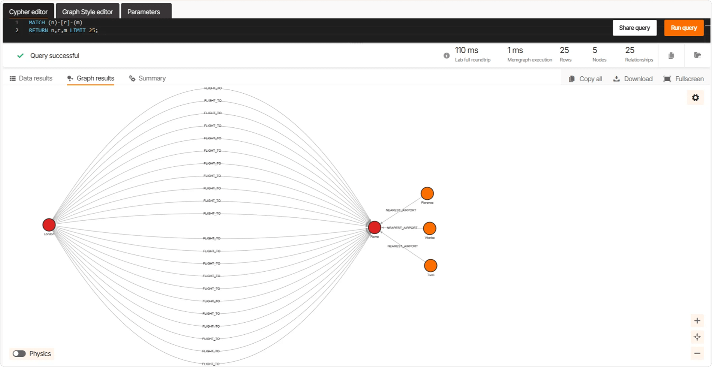
The image below shows the results of a query which, due to a limit, displays only a part of the graph. You can clearly see flights from London to Rome, as well as the cities of Florence, Viterbo, and Tivoli, for which the Rome airport is the closest. This visualization helps in understanding the connections and relationships that our queries will explore in more detail.
Here is a list of list of queries we explored in this project:8
Query 1: List of all cities (with or without their own airport)
This first query is designed to generate a comprehensive list of all cities available in the database, which would be ideal for populating a flight search application's user interface.
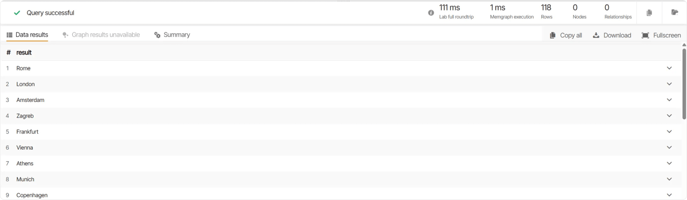
It accomplishes this by searching for both :City and :Airport nodes and extracting the city name from them. The result is a list of all cities in the database.
MATCH (n)
RETURN CASE
          WHEN n:City THEN n.name
          WHEN n:Airport THEN n.city
          ELSE NULL
       END AS result;
In the image below, we can see the output of this query, showing that 118 cities are stored in this database.
Query 2: Finding the nearest airport for departure and destination cities
The purpose of this query is to find the correct airport codes for cities entered by a user, working for both cities that have their own airport and those that don't. The query intelligently finds the nearest airport for a given city and retrieves its code.
For example, when given the cities "Čakovec" and "Versailles," the query returns the corresponding airport codes ZAG (Zagreb) and CDG (Paris), as shown below.
Query:
// subquery for all subsequent queries
WITH "Cakovec" AS departureCity, "Versailles" AS destinationCity

MATCH (departureNode)
WHERE (departureNode:City AND departureNode.name = departureCity) OR (departureNode:Airport AND departureNode.city = departureCity)
OPTIONAL MATCH (departureNode:City)-[rDep:NEAREST_AIRPORT]->(nearestDepartureAirport:Airport)
WITH departureCity, destinationCity,
     departureNode, nearestDepartureAirport, rDep
MATCH (destinationNode)
WHERE (destinationNode:City AND destinationNode.name = destinationCity) OR (destinationNode:Airport AND destinationNode.city = destinationCity)
OPTIONAL MATCH (destinationNode:City)-[rDest:NEAREST_AIRPORT]->(nearestDestinationAirport:Airport)
WITH
    CASE
        WHEN departureNode:Airport THEN departureNode.code
        ELSE nearestDepartureAirport.code
    END AS departureAirportCode,
    CASE
        WHEN destinationNode:Airport THEN destinationNode.code
        ELSE nearestDestinationAirport.code
    END AS destinationAirportCode,
    departureNode,
    destinationNode,
    nearestDepartureAirport,
    nearestDestinationAirport,
    rDep,
    rDest

RETURN departureAirportCode, destinationAirportCode;
Response:
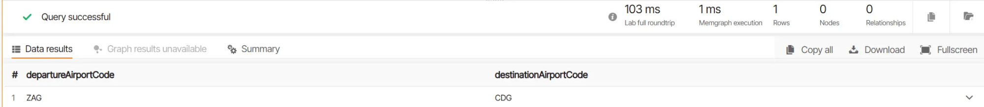
This functionality ensures that the application can always provide flight options, even for smaller cities. This query will also be used as a subquery for all subsequent flight-finding queries.
Query 3: Cheapest direct flight
This query is all about finding the cheapest direct flight between two cities, such as "Čakovec" and "Eisenstadt."
It's a great example of how a graph database can handle a common scenario where travelers are searching for flights and want to sort the results by price.
The query first uses a subquery to figure out the right airport codes for each city and then finds the direct flight between them. It returns a full breakdown of the flight details, from the airline and flight times to the price and duration.
// Using the airport codes from the second query
MATCH path=(n {code: departureAirportCode})-[r:FLIGHT_TO]->(m {code: destinationAirportCode})
RETURN
    departureNode,
    CASE WHEN rDep IS NOT NULL THEN [departureNode, rDep, nearestDepartureAirport] ELSE [] END AS departureToAirportPath,
    destinationNode,
    CASE WHEN rDest IS NOT NULL THEN [destinationNode, rDest, nearestDestinationAirport] ELSE [] END AS destinationToAirportPath,
    nodes(path) AS directFlightNodes,
    relationships(path) AS directFlightRelationship,
    r.durationMinutes AS flightDuration,
    r.priceEur AS flightPrice,
    r.departureTimestamp AS departureTime,
    r.arrivalTimestamp AS arrivalTime
ORDER BY r.priceEur ASC
LIMIT 1;
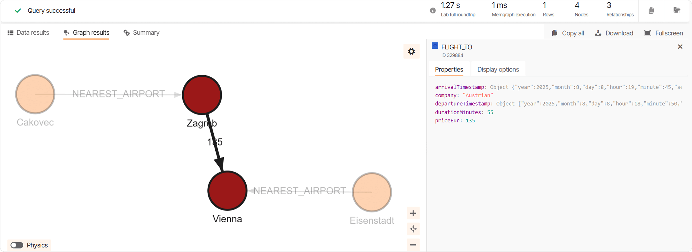
The result suggests a flight from Zagreb to Vienna on August 8, 2025 for just 135 euros, as shown in the image below.
Query 4: Cheapest Flight With Possible Layovers and A Maximum of 2 Days of Total Travel Time
This query is designed to find the cheapest flight between two cities, like Čakovec and Eisenstadt, with a few clever conditions. It's perfect for flexible travelers who are prioritizing cost over travel time.
The query uses a weighted shortest path algorithm, where the "weight" is the price of each flight, and it allows for an unlimited number of layovers. To keep the results realistic, it adds constraints ensuring that the total travel time doesn't exceed two days and that connections are valid.
// Using the airport codes from the second query
MATCH path=(n {code: departureAirportCode})-[:FLIGHT_TO *WSHORTEST (r, n | r.priceEur) totalPrice
  (r, n, p, w |
    size(relationships(p)) <= 1 or
    ((relationships(p)[-2]).arrivalTimestamp < r.departureTimestamp) and
    (relationships(p)[0]).arrivalTimestamp.day + 2 > r.departureTimestamp.day
  )]->(m {code: destinationAirportCode})
RETURN
    departureNode,
    CASE WHEN rDep IS NOT NULL THEN [departureNode, rDep, nearestDepartureAirport] ELSE [] END AS departureToAirportPath,
    destinationNode,
    CASE WHEN rDest IS NOT NULL THEN [destinationNode, rDest, nearestDestinationAirport] ELSE [] END AS destinationToAirportPath,
    nodes(path) AS shortestPathNodes,
    relationships(path) AS shortestPathRelationships,
    totalPrice;
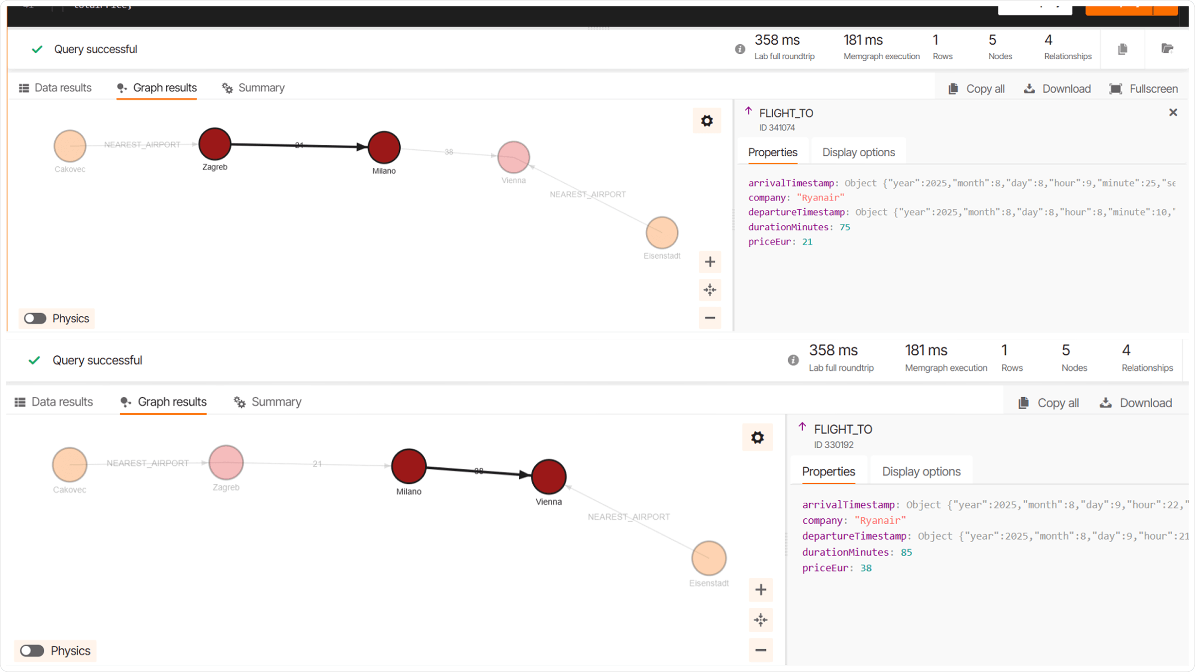
For our example, the query finds a route with a single layover in Milan: a flight departing from Zagreb on August 8th and a connecting flight from Milan to Vienna on August 9th. The total price for this route is 59 Euros, which is less than half the cost of the direct flight found in our previous query. The result of the query is shown below:
Query 5: Shortest Flight by Duration With Possible Layovers and a Maximum of 1 Day of Total Travel Time
The final query is designed to find the fastest possible route between two cities, in this case, Zagreb and Porto, within a strict one-day travel limit.
This is a perfect example for business travelers who need to minimize travel time above all else. The query uses a weighted shortest path algorithm, where the "weight" is the duration of each flight in minutes, to find the quickest route.
// Using the airport codes from the second query for cities Zagreb and Porto
MATCH path=(n {code: departureAirportCode})-[:FLIGHT_TO *WSHORTEST (r, n | r.durationMinutes) totalDuration
  (r, n, p, w |
    size(relationships(p)) <= 1 or
    ((relationships(p)[-2]).arrivalTimestamp < r.departureTimestamp) and
    (relationships(p)[0]).arrivalTimestamp.day + 1 > r.departureTimestamp.day
  )]->(m {code: destinationAirportCode})
RETURN
    departureNode,
    CASE WHEN rDep IS NOT NULL THEN [departureNode, rDep, nearestDepartureAirport] ELSE [] END AS departureToAirportPath,
    destinationNode,
    CASE WHEN rDest IS NOT NULL THEN [destinationNode, rDest, nearestDestinationAirport] ELSE [] END AS destinationToAirportPath,
    nodes(path) AS shortestPathNodes,
    relationships(path) AS shortestPathRelationships,
    totalDuration;
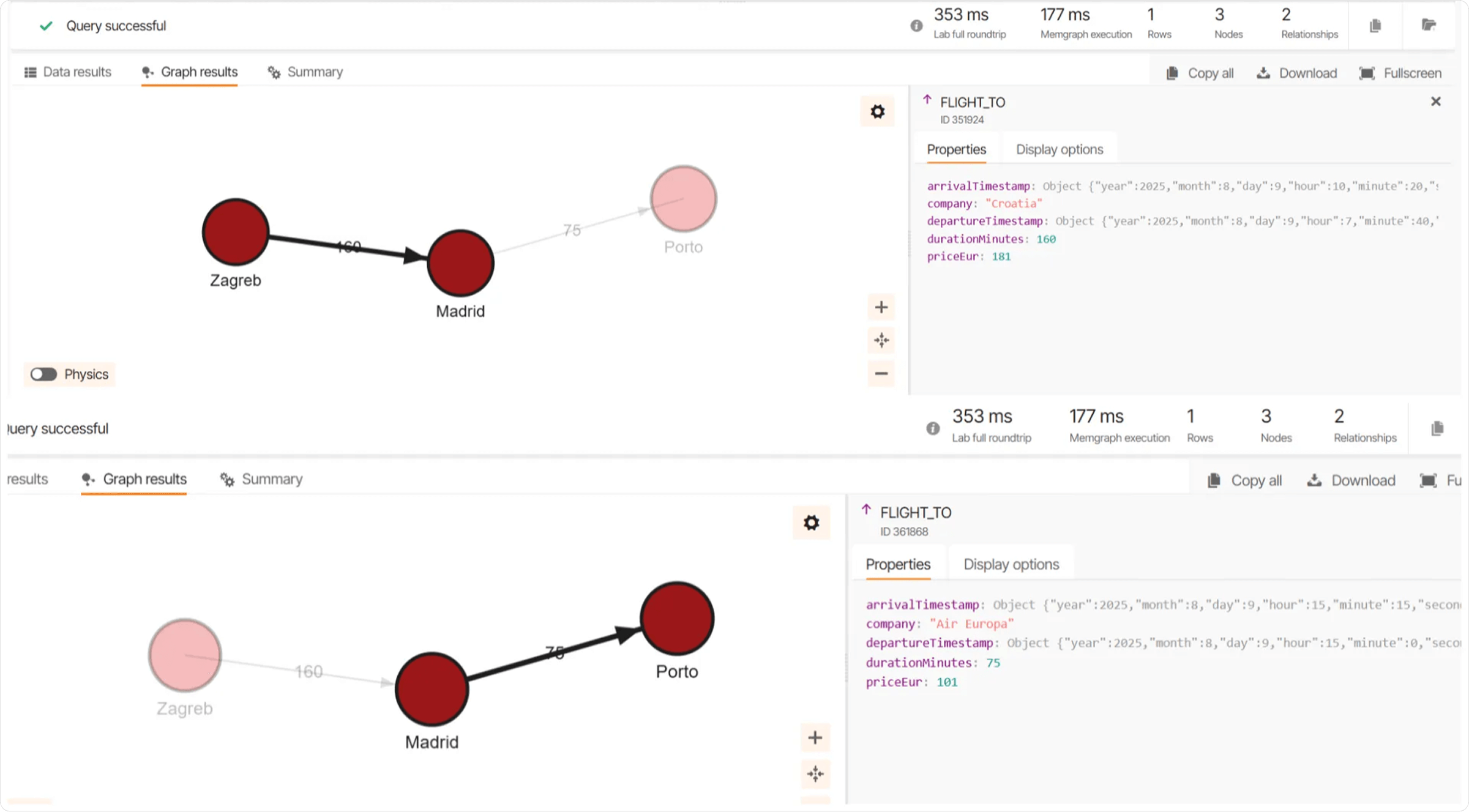
Since there are no direct flights between Zagreb and Porto, the query finds a route with a layover in Madrid. The result is a total travel time of 3 hours and 55 minutes, with a flight from Zagreb to Madrid on August 9th and a connecting flight from Madrid to Porto later the same day. The result of the query is shown below.
Wrapping Up
And just like that, we've completed this project!
We've demonstrated how a flight search engine can be built with the Memgraph graph database and Cypher queries, turning complex flight data into a powerful tool for finding optimal travel routes. This approach makes navigating a web of connections feel as simple as a few clicks, proving that Memgraph is the perfect co-pilot for any project involving interconnected data.
For future adventures, the system could easily be expanded to include other forms of transportation, like trains, creating the ultimate travel-planning experience.
Happy travels, and may your next connection always be on time!