How to Read the Query Execution Plans to Optimize Your Queries

Running an optimized database query involves understanding a query language that gets translated into the query plan suitable for your database. However the underlying principle of optimizing any query or algorithm is computational complexity. That’s where we’ll start.

Computational complexity

Although the words complex and complicated may appear identical terms to an average speaker to a computer science guru, in the context of computation and software, the two have almost nothing in common. Computational complexity is commonly known as a measure of how a piece of software, module, algorithm, or function scales performance-wise regarding inputs. The focus often is on one type of computational complexity, called time complexity.

Not to spend too much time defining both terms since they are one of the hardest topics in computer science, let’s rather break the time complexity down.

There are only two hard things in Computer Science: cache invalidation and naming things. -- Phil Karlton

Time complexity

To avoid this being an abstract topic, let’s put things into a practical perspective: imagine you have a query you need to execute in your software infrastructure. There are 1k users in the database. You need to find all the users whose names start with the letter A and who are above 27 years old to update their account balance. Apparently, when dealing with 1,000 records or nodes, your system can execute and process requests in just 0.1 seconds. Now, that seems fine at that scale, but what happens once you have more users?

The question is how much time will it take to execute this on 10k users in the database? If there are 100k users, will it be 10 seconds? That is what time complexity defines, providing a rough estimate of how scalable the processing request is.

Now imagine that your query has a linear complexity, meaning, for 10k users, it will take 1 second, while for 100k users — 10 seconds. That does not seem as scalable, right? By buying a twice-as-fast processing server, you can split that time in half, but hardware is not cheap, and there is a limit on available hardware.

Although the wall clock time is often what matters to customers and humans waiting for a query to finish, computer scientists use a different way of defining time complexity.

Big O notation

So, the time complexity should help us understand how complex a query or algorithm is, which directly defines how much time it takes a computer to run it. But how do we go about defining this complexity? Saying it takes a second is invalid: if the hardware can run the query 2 times faster, it will execute in half a second. So, both results, although different, are not comparable on different hardware.

To avoid this hardware dependency, developers refer to the Big O notations that define limiting behaviors. Take a look at the following graph:

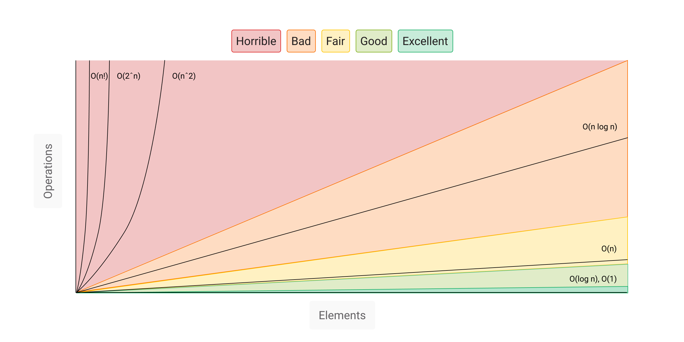
So, the vertical axis represents the number of operations or steps needed to compute something, while the horizontal axis represents the number of elements n. So the O(n) reads as “Big O of n,” which means that the query marked as O(n) has linear complexity since that function grows linearly.

As previously mentioned, a query has a linear complexity O(n): it takes 0.1 second to run 1k nodes and 1 second — for 10k nodes. This is a linear growth rate.

Let’s say that the query has a quadratic complexity O(n^2). As the number of elements n increases, the growth rate of the number of operations grows in a quadratic manner, which quickly goes out of hand.

Here is a table for some dummy algorithms running on different scales:

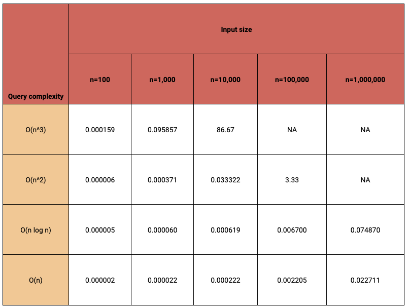
As you can see in the table, quadratic and cubic complexities are not usable at all for above 100k users. Keep in mind that these are just numbers for simplification and understanding query complexity. Here is an article to understand time-complexity and Big O.

So, what do query complexity and query plans have in common?

Memgraph query plans

Before they are run, if the database system has declarative query language, such as SQL or Cypher, the query is translated into the query plan first. The query plan defines steps to execute, which yield the query's computational complexity.

Query plan

A query plan (or query execution plan) is a sequence of steps used to access data in a database storage engine. Not all plans are the same, and you can have different query plans for identical queries, depending on the configuration of the database.

Think of this query execution plan as a pipeline. It’s essentially a sequence of logical operators that process data step by step, moving it from one operator to the next. To peek under the hood and understand how your query will be executed, prefix your query with the EXPLAIN clause. This lets you view the generated plan, providing a clearer understanding of the query execution pathway.

First, load the database with the data you have and run this simple query:

EXPLAIN MATCH (n) RETURN n;

Here is the basic example of a query plan:

+------------------+
| QUERY PLAN       |
+------------------+
| " * Produce {n}" |
| " * ScanAll (n)" |
| " * Once"        |
+------------------+

The query plans are meant to be read from the bottom to the top. This simple query has three steps in a query plan:

Once - Forms the beginning of an operator chain with "only once" semantics. The operator will return false on subsequent pulls.

ScanAll (n) - Produces all nodes in the database.

Produce {n} - Produces results.

This gives you an understanding of what the database is doing in the background, yet the question is what each operator does and how complex it is.

To get time details and performance information, use the PROFILE clause, which provides a detailed performance report for the query plan.

PROFILE MATCH (n) RETURN n;

Here is the output:

+-----------------+-----------------+-----------------+-----------------+
| OPERATOR        | ACTUAL HITS     | RELATIVE TIME   | ABSOLUTE TIME   |
+-----------------+-----------------+-----------------+-----------------+
| "* Produce"     | 14578           | " 12.391340 %"  | "  1.480285 ms" |
| "* ScanAll"     | 14578           | " 87.607946 %"  | " 10.465755 ms" |
| "* Once"        | 2               | "  0.000714 %"  | "  0.000085 ms" |
+-----------------+-----------------+-----------------+-----------------+

OPERATOR: The operator’s designation, mirroring its name in an EXPLAIN query result. ACTUAL HITS: The number of times a particular logical operator was pulled. RELATIVE TIME: The time dedicated to a specific logical operator proportionate to the entire plan’s execution duration. ABSOLUTE TIME: The exact wall time duration spent processing a specific logical operator.

Before moving forward, note that for the rest of the blog post, we use a dataset with 14,579 nodes and 56,622 relationships.

You can use both the EXPLAIN and PROFILE clauses. The EXPLAIN clause returns the full query plan with operators, while the PROFILE clause returns all called operators and each operator’s performance-related information. Since the PROFILE clause provides more information, we’ll use it for the rest of the guide.

The implication of indexes

As previously mentioned, identical queries can have different query plans, which can result in different complexity and results. This is possible primarily because of indexes or database engine features. To put things into perspective, here is the example query:

PROFILE MATCH (n:Player) RETURN n;

Here is the output:

+-----------------+-----------------+-----------------+-----------------+
| OPERATOR        | ACTUAL HITS     | RELATIVE TIME   | ABSOLUTE TIME   |
+-----------------+-----------------+-----------------+-----------------+
| "* Produce"     | 4904            | "  6.230920 %"  | "  0.096880 ms" |
| "* Filter"      | 4904            | " 61.098997 %"  | "  0.949987 ms" |
| "* ScanAll"     | 14580           | " 32.667357 %"  | "  0.507923 ms" |
| "* Once"        | 2               | "  0.002726 %"  | "  0.000042 ms" |
+-----------------+-----------------+-----------------+-----------------+

The key information here is that we have ScanAll and Filter operators in the query plan; let’s see what happens when we add an index.

Now, setting the label index inside the database will change how the query gets executed:

CREATE INDEX ON :Player;

Running the same query again results in a different query plan:

EXPLAIN MATCH (n:Player) RETURN n;

Query plan:

+--------------------+--------------------+--------------------+--------------------+
| OPERATOR           | ACTUAL HITS        | RELATIVE TIME      | ABSOLUTE TIME      |
+--------------------+--------------------+--------------------+--------------------+
| "* Produce"        | 4904               | " 35.028645 %"     | "  0.135605 ms"    |
| "* ScanAllByLabel" | 4904               | " 64.959663 %"     | "  0.251475 ms"    |
| "* Once"           | 2                  | "  0.011692 %"     | "  0.000045 ms"    |
+--------------------+--------------------+--------------------+--------------------+

As you can see, the operator has changed from Filter and ScanAll to just ScanAllByLabel. In this particular case, indexes impacted the query execution and query running time: from 1.555 milliseconds to 0.357 milliseconds. The query engine changed a query plan based on the index configuration, resulting in optimization.

Indexes will play an important role in defining and optimizing your queries, The central part of our index data structure in Memgraph is a highly-concurrent skip list. Skip lists are probabilistic data structures that allow fast search within an ordered sequence of elements. The structure is built in layers, where the bottom layer is an ordinary linked list that preserves the order. Each higher level can be imagined as a highway for layers below.

Here are the implications of this data structure (n denotes the current number of elements in a skip list):

• The average insertion time is O(log(n))
• The average deletion time is O(log(n))
• The average search time is O(log(n))

As you can see O(log(n)) is logarithmic time, and this is much faster than linear time (refer to the image describing the Big O time complexity).

Creating indexes and using them will enable your queries to become more scalable. Of course, there are some tradeoffs with indexes, such as requiring extra storage (memory) for each index and slowing down write operations in the database.

Optimizing your queries through Memgraph

Based on everything mentioned so far, you should have built a mental model of how to approach the issue of complexity and the implication of indexes. Let’s go over a few examples of optimization steps that will help you pass that on to your queries.

Memgraph operators in a query plan

Memgraph has a long list of operators that can be used in the query plan; in this blog post, we will focus on the ones interacting with indexes, which are the following:

Operator Description ScanAll Produces all nodes in the database. ScanAllByLabel Produces nodes with a certain label. ScanAllByLabelPropertyValue Produces nodes with a certain label and property value.

For the full list, head over to Memgraph’s docs. Optimizing the query plan

Let’s start with a simple query and no indexes to see the impact.

PROFILE MATCH (n:Transfer{year:1992}) RETURN n;

+-----------------+-----------------+-----------------+-----------------+
| OPERATOR        | ACTUAL HITS     | RELATIVE TIME   | ABSOLUTE TIME   |
+-----------------+-----------------+-----------------+-----------------+
| "* Produce"     | 148             | "  0.124672 %"  | "  0.011513 ms" |
| "* Filter"      | 148             | " 55.090997 %"  | "  5.087585 ms" |
| "* ScanAll"     | 14578           | " 44.783428 %"  | "  4.135694 ms" |
| "* Once"        | 2               | "  0.000903 %"  | "  0.000083 ms" |
+-----------------+-----------------+-----------------+-----------------+

As you can see, this will have typical Once and Produce operators, which are unimportant since they take less than 1% of the time. Operators Filter and ScanAll take almost all of the time, and notice that both operators’ ACTUAL HITS and ABSOLUTE TIME values make 99% of the relative time. In this particular case, the ScanAll has linear complexity since it needs to go over all the nodes in the database, resulting in 14 578 nodes. After that, Filter does the filtering on each node from ScanAll. Although we did specify the label :Transfer for nodes, it didn’t help. This is because Memgraph does not contain label indexes by default.

To improve on this ScanAll, we can set the label index on :Transfer:

CREATE INDEX ON :Transfer;

Now, after running a query again:

PROFILE  MATCH (n:Transfer{year:1992}) RETURN n;

Here is the result:

+--------------------+--------------------+--------------------+--------------------+
| OPERATOR           | ACTUAL HITS        | RELATIVE TIME      | ABSOLUTE TIME      |
+--------------------+--------------------+--------------------+--------------------+
| "* Produce"        | 148                | "  0.295283 %"     | "  0.015274 ms"    |
| "* Filter"         | 148                | " 39.778457 %"     | "  2.057557 ms"    |
| "* ScanAllByLabel" | 9438               | " 59.926260 %"     | "  3.099711 ms"    |
| "* Once"           | 2                  | "  0.000000 %"     | "  0.000000 ms"    |
+--------------------+--------------------+--------------------+--------------------+

Immediately, you can notice the operator changed from ScanAll to ScanAllByLabel, a drop in actual hits, and of course, the execution time. From an initial iteration of 9 milliseconds, the query now takes 5 milliseconds.

If you look at the first results, you will notice that Filter is now also twice as fast because it has fewer nodes to process since ScanAllByLabel is producing roughly 9k nodes while ScanAll is producing all 14k nodes. Having a label index will help massively if you have a nice graph model where labels are in a nice balance.

But if you take a look at the query, we did specify the year that is being filtered. If there is a property that’s very important for queries, you should consider creating an index on that property.

Run the following index creation:

CREATE INDEX ON :Transfer(year);

Then run the same query again:

PROFILE MATCH (n:Transfer{year:1992}) RETURN n;

+---------------------------------+---------------------------------+---------------------------------+---------------------------------+
| OPERATOR                        | ACTUAL HITS                     | RELATIVE TIME                   | ABSOLUTE TIME                   |
+---------------------------------+---------------------------------+---------------------------------+---------------------------------+
| "* Produce"                     | 148                             | " 14.396015 %"                  | "  0.049264 ms"                 |
| "* ScanAllByLabelPropertyValue" | 148                             | " 85.579078 %"                  | "  0.292858 ms"                 |
| "* Once"                        | 2                               | "  0.024907 %"                  | "  0.000085 ms"                 |
+---------------------------------+---------------------------------+---------------------------------+---------------------------------+

Now notice that in the query plan, the ScanAllByLabelPropertyValue operator is doing all of the processing, next to Once and Produce, of course. The actual hits now dropped to 148 nodes, and the query is executed within 0.3 milliseconds, which is 30 times faster than without indexes. Generally speaking, having a shorter query plan and fewer hits will yield better results. Keep that in mind when debugging queries.

Queries can have a slightly different structure and still be executed the same; this is why checking the query plan is important from an optimization point of view. If you rewrite the previous query a bit, like this:

PROFILE  MATCH (n:Transfer) WHERE n.year = 1992 RETURN n;

It will result in the same query plan and will be executed the same way as in the previous step.

+---------------------------------+---------------------------------+---------------------------------+---------------------------------+
| OPERATOR                        | ACTUAL HITS                     | RELATIVE TIME                   | ABSOLUTE TIME                   |
+---------------------------------+---------------------------------+---------------------------------+---------------------------------+
| "* Produce"                     | 148                             | "  8.121183 %"                  | "  0.043120 ms"                 |
| "* ScanAllByLabelPropertyValue" | 148                             | " 91.862955 %"                  | "  0.487754 ms"                 |
| "* Once"                        | 2                               | "  0.015862 %"                  | "  0.000084 ms"                 |
+---------------------------------+---------------------------------+---------------------------------+---------------------------------+

You can still fool your query planner. Here is an example:

PROFILE  MATCH (n:Transfer) WHERE n.year IS NOT NULL AND n.year = 1992 RETURN n;

So, in this particular case, we did write a condition where the year is not null and the year is 1992. Obviously, checking for the year not to be NULL is useless here since the year has a value in that condition.

Here is the result of running that query:

+---------------------------------+---------------------------------+---------------------------------+---------------------------------+
| OPERATOR                        | ACTUAL HITS                     | RELATIVE TIME                   | ABSOLUTE TIME                   |
+---------------------------------+---------------------------------+---------------------------------+---------------------------------+
| "* Produce"                     | 148                             | "  2.377972 %"                  | "  0.011162 ms"                 |
| "* Filter"                      | 148                             | " 13.525836 %"                  | "  0.063487 ms"                 |
| "* ScanAllByLabelPropertyValue" | 148                             | " 84.078312 %"                  | "  0.394643 ms"                 |
| "* Once"                        | 2                               | "  0.017879 %"                  | "  0.000084 ms"                 |
+---------------------------------+---------------------------------+---------------------------------+---------------------------------+

This condition nudged the query planner to introduce a filter check, which is unnecessary and takes 13% of the time in this case. So, try to write the most compact version of the queries. In the meantime, we will work on improving the query interpreter and Memgraph in general.

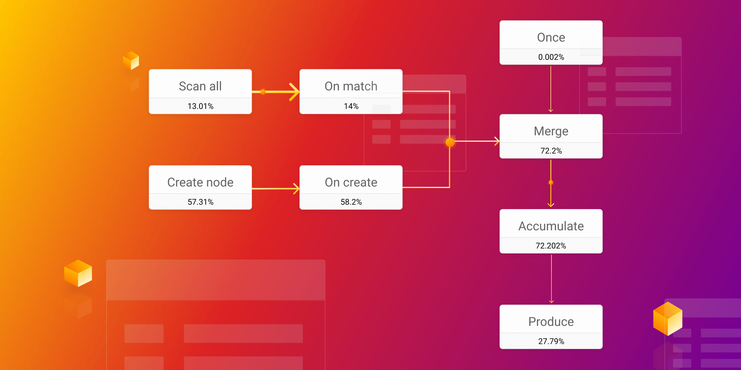
Everything mentioned applies to the write queries in the database, they can also be index-dependent. The MERGE query is an example of this since it first needs to search, and then, depending on the search result, it will write something to the database. Here is an example:

PROFILE MERGE (p:Player{name:"Pele"}) RETURN p

Not having a proper label and property index will result in the following summary:

+------------------+------------------+------------------+------------------+
| OPERATOR         | ACTUAL HITS      | RELATIVE TIME    | ABSOLUTE TIME    |
+------------------+------------------+------------------+------------------+
| "* Produce"      | 2                | "  0.036516 %"   | "  0.004136 ms"  |
| "* Accumulate"   | 2                | "  0.500531 %"   | "  0.056686 ms"  |
| "* Merge"        | 2                | "  0.260409 %"   | "  0.029492 ms"  |
| "|\\"            | ""               | ""               | ""               |
| "| * Filter"     | 1                | " 57.750671 %"   | "  6.540384 ms"  |
| "| * ScanAll"    | 14578            | " 40.370400 %"   | "  4.572032 ms"  |
| "| * Once"       | 2                | "  0.000369 %"   | "  0.000042 ms"  |
| "|\\"            | ""               | ""               | ""               |
| "| * CreateNode" | 1                | "  1.080365 %"   | "  0.122354 ms"  |
| "| * Once"       | 1                | "  0.000369 %"   | "  0.000042 ms"  |
| "* Once"         | 2                | "  0.000369 %"   | "  0.000042 ms"  |
+------------------+------------------+------------------+------------------+

As you can see, 97% of the query time execution is spent in ScanAll and Filter operators, while the creation of the query takes just 1% of the time. Setting label and property index will result in the following optimized query plan:

+-----------------------------------+-----------------------------------+-----------------------------------+-----------------------------------+
| OPERATOR                          | ACTUAL HITS                       | RELATIVE TIME                     | ABSOLUTE TIME                     |
+-----------------------------------+-----------------------------------+-----------------------------------+-----------------------------------+
| "* Produce"                       | 2                                 | "  3.853928 %"                    | "  0.012310 ms"                   |
| "* Accumulate"                    | 2                                 | " 64.169249 %"                    | "  0.204967 ms"                   |
| "* Merge"                         | 2                                 | "  3.180164 %"                    | "  0.010158 ms"                   |
| "|\\"                             | ""                                | ""                                | ""                                |
| "| * ScanAllByLabelPropertyValue" | 1                                 | " 11.790864 %"                    | "  0.037662 ms"                   |
| "| * Once"                        | 2                                 | "  0.013475 %"                    | "  0.000043 ms"                   |
| "|\\"                             | ""                                | ""                                | ""                                |
| "| * CreateNode"                  | 1                                 | " 16.965369 %"                    | "  0.054190 ms"                   |
| "| * Once"                        | 1                                 | "  0.000000 %"                    | "  0.000000 ms"                   |
| "* Once"                          | 2                                 | "  0.026951 %"                    | "  0.000086 ms"                   |
+-----------------------------------+-----------------------------------+-----------------------------------+-----------------------------------+

Wrapping up query execution plans

Each query you write gets interpreted to the query plan. In some cases, the same query can have different execution plans, and in others, different queries can be executed in the same way. This can lead to different query performances depending on indexes and configuration options. To tackle this, it is necessary to check the query execution plans and optimize your paths as much as possible.

If you have issues optimizing your queries, we are always open to help! Give us a nudge on our Discord server to also become a part of the community.