How Node2Vec Works – A Random Walk-Based Node Embedding Method

Introduction

In this article, we will try to explain a node embedding random walk-based method called node2vec.

If you are not familiar with embeddings, we prepared a blog post on the topic of node embeddings. There, you can learn what node embeddings are, where we use them and how to generate them from a graph.

Node2Vec idea

Node2Vec is a random walk-based node embedding method developed by Aditya Grover and Jure Leskovec.

Do you remember why we use walk sampling?

If the answer is no, feel free to check the blog post on node embeddings, especially the part on random walk-based methods, where we explained the similarity between walk sampling in random walk-based methods and sentences that are used in word2vec.

For node2vec, the paper authors came up with the brilliant idea:

We define a flexible notion of a node’s network neighborhood and design a biased random walk procedure, which efficiently explores diverse neighborhoods.

This sounds interesting. It means that at any point in the walk, we roll a dice to decide which edge will be the next in our walk, leading to a new node. In node2vec, walk sampling is not random, but depends on two hyperparameters that add bias to the walk sampling:

• p - the return parameter
• q - the in-out parameter

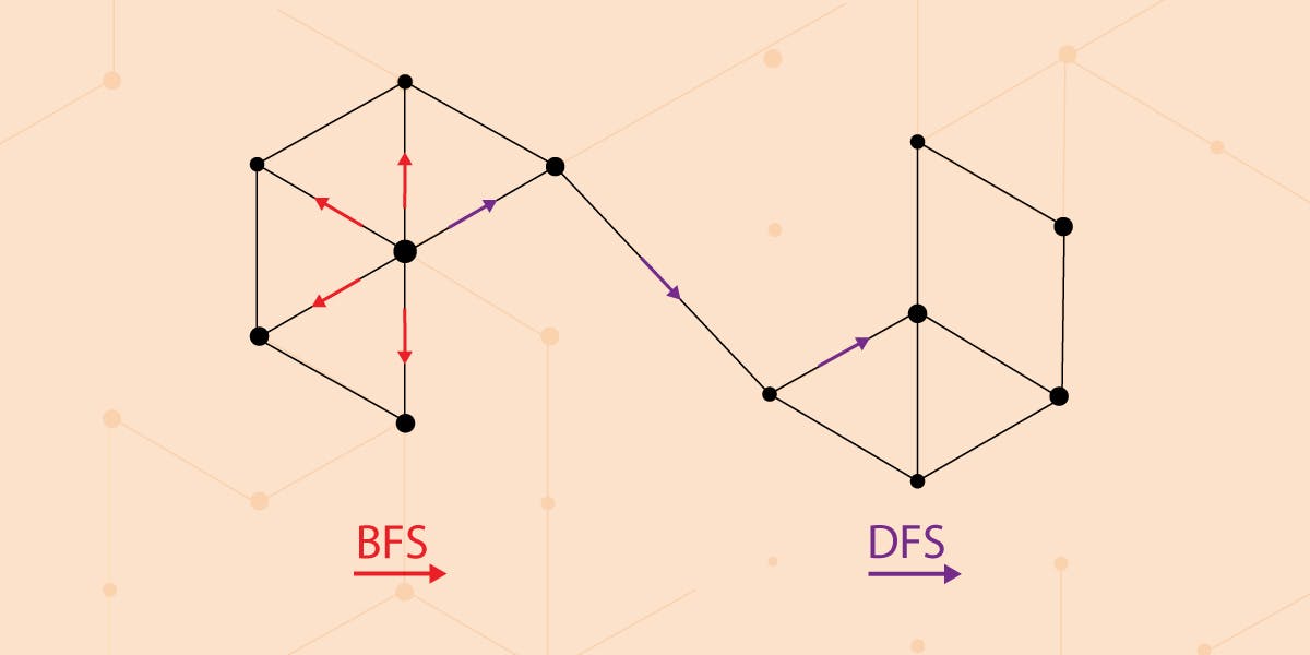
From the picture below, you maybe get the idea of how we achieve "a flexible notion of a node’s network neighborhood" and how p and q influence the walk sampling. We still didn't start with the explanation, so don't worry, everything will be explained.

Before we start with an explanation of the node2vec algorithm, let's divide it into 3 unique steps:

• 1. Edge transition probability calculation
• 2. Walk sampling
• 3. Embedding calculation

What is so great about this algorithm is that each step is parallelizable.

Edge transition probability calculation

In order to sample a walk, we move from one node to another in the direction of the edge. If the edge is undirected, you can move in any direction across the edge. Hang on, this will be important later on.

Have you heard of the terms homophily equivalence and structural equivalence? It was shown in a research paper that prediction tasks in networks, such as link prediction, node classification, and so on, often vary between these two equivalences. Under the homophily hypothesis, nodes that are highly interconnected and belong to similar network clusters (communities) should be embedded closely together. In contrast, under the structural equivalence hypothesis, nodes that have similar structural roles (like hubs for example) in networks should be embedded closely together. What is more important is nodes could be far apart in the network and still have the same structural role.

And now for the really cool part. It was observed in a research paper that BFS and DFS have a key role in producing representations that reflect either of the above equivalences (homophily or structural equivalence). The neighborhoods sampled by BFS lead to embeddings that correspond closely to structural equivalence. It is because in order to find structural equivalence it is sufficient to characterize the local neighborhoods accurately. BFS achieves this easily since it first explores around nodes by obtaining a microscopic view of the network. On the other hand, DFS can explore larger parts of the network as it can move further away from the source node from which we started walk sampling. And with DFS, nodes more accurately reflect the macro-view of the network which is essential in inferring communities, homophily equivalence.

Back to the parameters p and q. By setting the different values of parameters before the walk sampling begins, you can achieve more BFS or DFS like walks. This means that with one algorithm, you can find communities in a graph or hubs.

How do we achieve such a task?

In order to introduce BFS and DFS like walks, we first need to introduce the concept of bias in random walks. This means our walk sampling will not anymore be totally random, but it will tend to behave in a certain way, like a biased coin.

The simplest way to bias our random walk is by edge weights. Every edge in a graph has some initial weight. Weights often represent how strong a connection between two nodes is, or how similar they are. Let's formalize the mathematical concept of bias with edge weights. Given some edge weight wᵤᵥ between nodes u and v, we can say that the transition probability from node u to node v is πᵤᵥ=wᵤᵥ. If the graph is undirected, the same accounts for the transition from node v to node u. Back to normal language, we just gave an initial definition of transition probability from one node to the other. If we were to make a sum Z of all transition probabilities from one node u to its neighborhood nodes vᵢ and divide each edge transition probability with that sum, we would have a normalized transition probability from one node to its neighbors. For better understanding, take a look at the picture below ⬇️

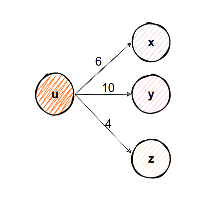
Take a look at the node u. The sum Z of all edge weights from node u is Z=20. In order to find the probability of moving from node u to any other node (v, x, y), we can divide each edge weight wᵤᵥ=6, wᵤₓ=10, wᵤᵧ=4 with 20, and we will get wᵤᵥ=0.3, wᵤₓ=0.5, wᵤᵧ=0.2. These are now normalized weights because their sum is 1, and here Z was the normalizing constant. How can we use these normalized edge weights? Each edge weight can represent a probability to move from node u to another node. And now when doing walk sampling, there would be a 50% possibility we would move to node x, 30% to move to node v, and only 20% to move to node y if we were on node u. And by doing so for every node, we introduced the concept of bias.

Now, you can still see that this does not allow us to account for the network structure and guide our search procedure to explore different types of network neighborhoods. This is where p and q come in place.

Parameters p and q

Let's first define what parameters p and q mean and then we will explain how they work on a simple case:

• p - also called the return parameter. It controls the likelihood of immediately returning to a node we just visited in a walk.
• q - the in-out parameter. It controls how likely we are to stay in the neighborhood of node u, or are we more likely to visit nodes further away from node u.

From this, you can see that p and q are intertwined. The value of one doesn't alone tell us how the walk sampling will be performed.

We don't use p and q directly, but 1/p and 1/q. Till now, our unnormalized transition probability was πᵤᵥ=wᵤᵥ. From now on, our unnormalized transition probability will be πᵤᵥ=α(t,v) * wᵤᵥ.

What does this parameter α(t,v) mean, and what's the new node t in this equation?

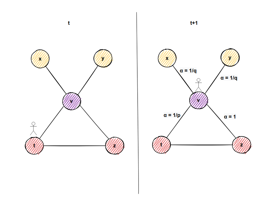
Imagine you are traveling through the graph. From node t, there needs to be an edge to node u (node on which we are on now), and also there is an edge from node u to node v (neighborhood node of node u). Furthermore, there might be an edge from node v (neighborhood of node u), to node t (node we came from to node u). Again, a picture to clarify things:

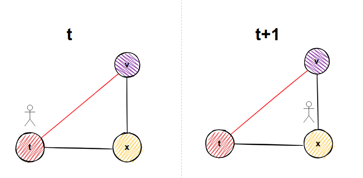
In the figure above, imagine we came from node t to the node u. There might be an edge from node v to node t. That means if we go to node v, in the next step, we might visit node t again in our current walk. For every neighbor of node u (don't forget that includes node t we came from if the graph is undirected), we have the following simple formula below to determine transition probabilities:

• If there is no edge from node v to node t, then transition probability πᵤᵥ = wᵤᵥ * 1/q. This is example 1 in our picture below.
• If there is an edge from node v to node t, then transition probability πᵤᵥ = wᵤᵥ * 1. This is example 2 in our picture below.
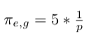
• No matter whether there is an edge or there is no edge from node v to node t, the transition probability is πₜᵤ=wₜᵤ * 1/p since it is our start node. These are examples 3 and 4 in the picture below.

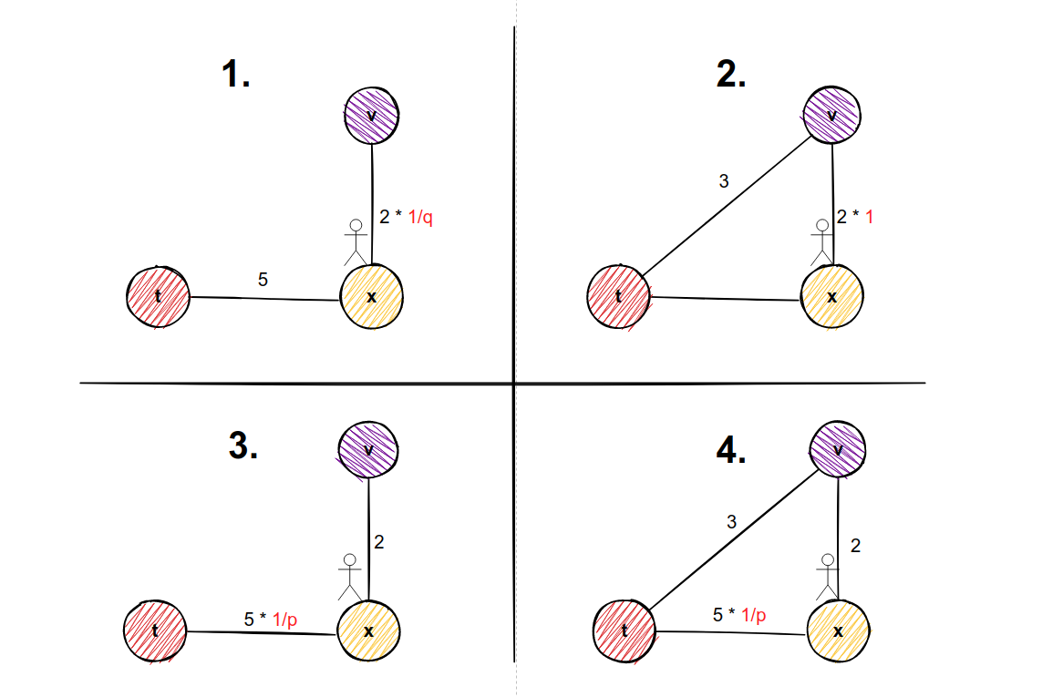
Why in example 1 we multiply edge weight with 1/q and in example 2 we multiply edge weight with factor 1?

If we want to sample nodes in a more DFS like manner, then we would want to explore nodes far away from our starting node. And we would make our parameter q very small because 1/q would be a big number, which equals to greater possibility to move away from starting node. But if we can return to our starting node t from potential node v, then we don't want to give the greater possibility to that transition.

Now, we repeat the following process for every edge. If the graph is undirected, we calculate probabilities for both directions.

Considering the normalization constant, it will be different for every edge and it will matter from which node we came from, and on which node we are now.

Example of calculating transition probabilities

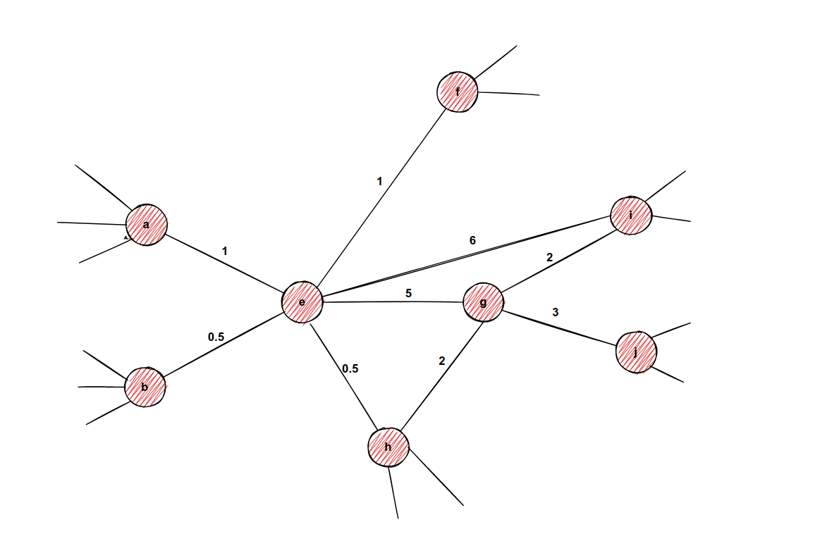
Imagine we are processing edge e-g in an undirected graph, and imagine we have the following weights the from picture. Weights don't need to be normalized just yet.

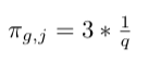
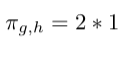
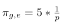
1. In this part of the example, we are calculating transition probabilities for node g, by arriving from node e. The neighbors of node g are nodes i, j, h, and e. The math looks like this:

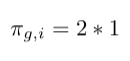
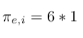
   • Multiply weight with factor 1 since there is return edge from node i to node e:
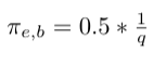
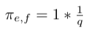
   • Multiply weight with factor 1/q since there is no edge from j to node e:
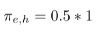
   • Multiply weight with factor 1 since there is a return edge from node h to node e:
   • Multiply weight with factor 1/p since it is our return node directly:

Then, we would calculate the sum of these transition probabilities and normalize each transition probability.

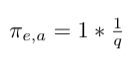
2. Next, we need to process the transition from g to node e too. Here, the math is a bit different:

   • Multiply weight with factor 1/q, since there is no return edge from node a to node g:
   • Multiply weight with factor 1/q since there is no edge from b to node g:
   • Multiply weight with factor 1/q since there is no return edge from node f to node g:
   • Multiply weight with factor 1 since there is return edge from node i to node g:
   • Multiply weight with factor 1 since there is return edge from node h to node g:
   • Multiply weight with factor 1/p since it is our return node directly:

Afterward, we hope you can get an idea of why it is called edge transition probability calculation. It depends on the edge we are on, and which direction we take. We just need to store this probability for every edge and every possible way of transition. These probabilities, once computed, will not change unless we add or remove a new edge.

Walk sampling

Since we calculated the transition probabilities, we can sample walks for every node. We are not doing this part by hand, we can use precomputed transition probabilities to sample our walk. For every edge, we make a biased coin flip to choose to which edge we will go next. After we have sampled num_walks walks and each one of the sampled walks had a maximum length of walk_length, our job here is done and we move on to the next step.

How to make embeddings of two nodes more similar?

These walks represent the neighborhood of a certain node. And we want to make our node embedding as similar as possible to embeddings of nodes in its neighborhood.

In math terms, this would mean the following: we seek to optimize the objective function which maximizes the logarithmic probability of observing a network neighborhood Nₛ(u) for node u based on its feature representation (representation in embedded space). Also, we make some assumptions for the problem to be easier to figure out. This is the formula:

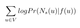
Here Pr(Nₛ(u)|f(u)) is the probability of observing neighborhood nodes of node u with the condition that we are currently in embedded space in place of node u. For example, if the embedded space of node u is the vector [0.5, 0.6], and imagine you are at that point, what is the likelihood to observe neighborhood nodes of node u. The goal is making the probability for every node as high as possible (that's why there is summation).

It sounds complicated, but with the following assumptions, it will get easier to comprehend:

1. The first one is that observing a neighborhood node is independent of observing any other neighborhood node given its feature representation. That means, in the "transitions" figure above, there is some probability for us to observe nodes x, y, and z if we are on node u currently. This is just relaxation for optimization used often in machine learning which makes it easier for us to compute the above mentioned probability Pr(Nₛ(u)|f(u)). The probabilities that we mentioned in the section Edge transition probability calculation are already incorporated in walk sampling.

2. The second one is that observing the source node and neighborhood node in the graph is the same as observing feature representation (embedding) of the source node and feature representation of the neighborhood node in feature space. Take a note that in the probability calculation Pr(Nₛ(u)|f(u)) we mentioned feature representation of node f(u) and regular nodes, which sounds like comparing apples and oranges, but with the following relaxation, it should be the same. So for some neighborhood node nᵢ in the neighborhood Nₛ of node u we could have the following:

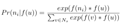
The exponential term is here so that the sum of probabilities of every neighborhood node of node u is 1. This is also called the softmax function.

Considering our optimization problem, this is it. Now, we hope that you get an idea what is our goal here. Luckily for us, this is already implemented in a Python module called gensim. Yes, these guys are brilliant in natural language processing and we will make use of it. 🤝

Conclusion

In this article, we covered what node2vec is and how it works. I hope you acquired a deeper understanding. ✍️

Our team of engineers is currently tackling the problem of graph analytics algorithms on real-time data. If you want to discuss how to apply online/streaming algorithms on connected data, feel free to join our Discord server and message us.

MAGE shares his wisdom on a Twitter channel. Get to know him better by following him 🐦

Last but not least, check out MAGE and don't hesitate to give a star ⭐ or contribute with new ideas.