Understanding How Dynamic node2vec Works on Streaming Data

Introduction

In this article, we will try to explain how node embeddings can be updated and calculated dynamically, which basically means as new edges arrive to the graph. If you still don't know anything about node embeddings, be sure to check out our blog post on the topic of node embeddings. 📖

There, we have explained what node embeddings are, where they can be applied, and why they perform so well. Even if you are familiar with everything mentioned, you can still refresh your memory.

Dynamic networks

Many methods, like node2vec and deepwalk, focus on computing the embedding for static graphs which is great but also has a big drawback. Networks in practical applications are dynamic and evolve constantly over time. New links are formed, and old ones can disappear. Moreover, new nodes can be introduced into the graph (e.g., users can join the social network) and create new links toward existing nodes.

How could one deal with such networks?

One idea could be to create a snapshot of a graph when a new edge is created [Leskovec et al., 2007]. Naively applying static embedding algorithms to each snapshot leads to unsatisfactory performance due to the following challenges:

• Stability: the embedding of graphs at consecutive time steps can differ substantially even though the graphs do not change much.
• Growing Graphs: All existing approaches assume a fixed number of nodes in learning graph embeddings and thus cannot handle growing graphs.
• Scalability: Learning embeddings independently for each snapshot leads to running time linear in the number of snapshots. As learning a single embedding is computationally expensive, the naive approach does not scale to dynamic networks with many snapshots

Dynamic Node2vec

Dynamic node2vec is a random-walk based method that creates embeddings for every new node added to the graph. For every new edge, there is a recalculation of probabilities (weights) that are used in walk sampling. A goal of the method is to enforce that the embedding of node v is similar to the embedding of nodes with the ability to reach node v across edges that appeared one before another. Don’t worry if this sounds confusing now, just remember that we have probability updates and walk sampling.

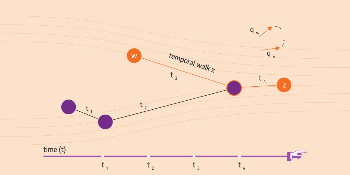
Take a look at Image 1. We sampled a walk as was mentioned before. By doing so, we created a list of nodes also known as temporal walk. The temporal part will be explained in a few seconds. And of course, the embedding of a node should be similar to the embedding of nodes in its temporal neighborhood. The algorithm itself consists of the following three parts in that order:

• 1) probabilities (weights) update
• 2) walk sampling
• 3) word2vec update

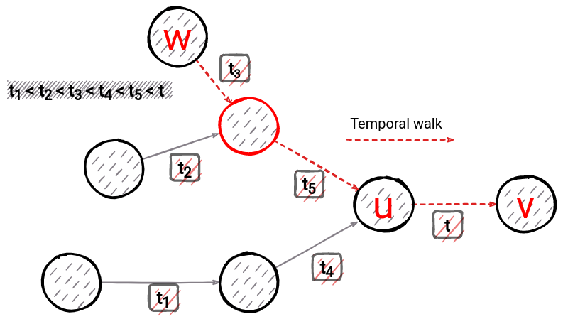
Few notes about terms we will use in the rest of the text. When a new directed edge is added to the graph it has source node and target node. Walk sampling means creating a walk through a graph. Every node we visit during walk sampling is memorized in order of visit. A walk can be constructed in a forward fashion, meaning we choose one of the out-going edges of a current node. Or it can be constructed in a backward fashion, which means we choose from one of the incoming edges of a current node. In backward walk sampling by choosing one of the incoming edges of the current node, we move to the new node, source node of that edge. And we repeat the step. The process for walk sampling in a backward fashion can be seen in Image 2. We start from node 9 and sampled walk looks as follows: 9,8,5,2,1. For example, when we were on the node with id 5, we could have chosen a different edge, which would take us to node 2, or node 4. Important: we are still not looking at the edge appearance timestamp, that is when has edge appeared in the graph.

We will first try to explain walk sampling, and then weight update, although in the real process they are reversed. We first do weight update, then walk sampling.

Walk sampling

In dynamic node2vec walks, sampling is done in time-dependent backward form. Backword sampling was explained before, so it's important you have a basic understanding for the next section.

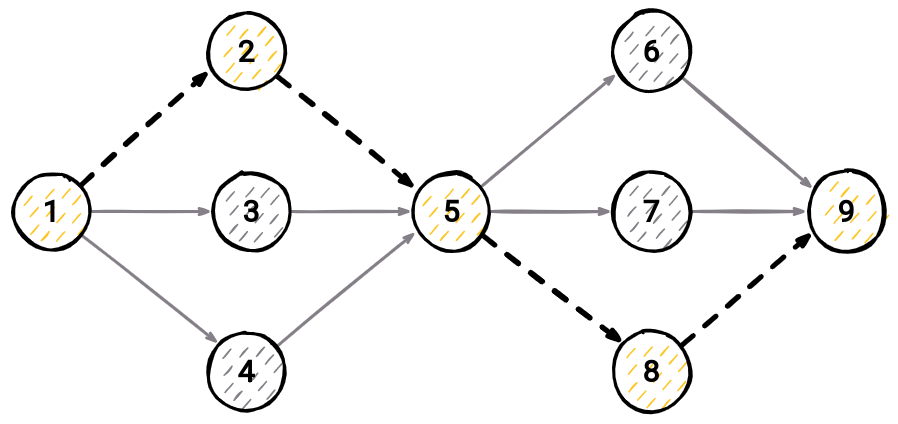
"Temporal" sampling means that from all possible incoming edges we only consider those that appeared before the last edge in the walk. Take a look at Image 3 and assume that we are on node 5. Since the last edge we visited was between nodes 5 and 8 (the edge is from 5 to 8, but we went from 8 to 5) appeared in the graph before edges 3⟶5 and 4⟶5, we can't even consider taking them as the next step. The only option is edge 2⟶5.

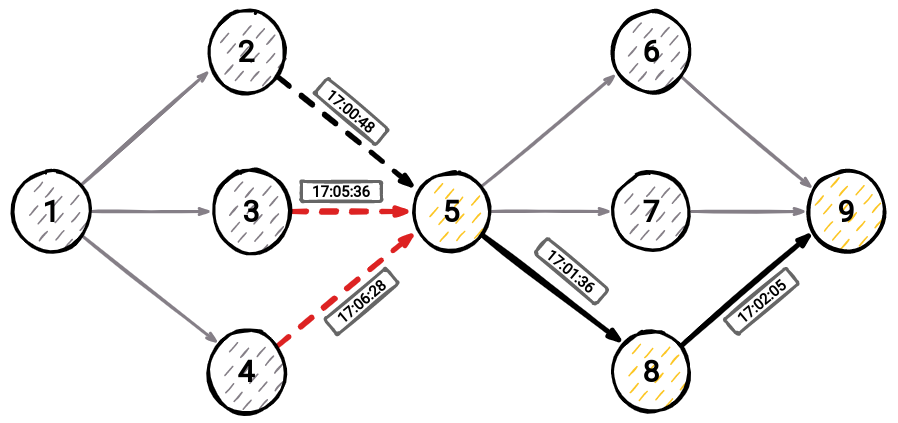
Since one node can have multiple incoming edges when sampling a walk, we use probabilities (weights) to determine which incoming edge of the node we will take next. It is like a biased coin flip. Take a look at Image 1. From node u you can take edge t4 or t5. When creating a walk, we want to visit nodes that were more recently connected by a new edge. They are carrying more information, therefore they have more importance to the graph than the old edges.

These probabilities are computed after the edge arrives and before temporal walk sampling (before this step). Walk sampling can be stopped, at any point, but at the latest when we sample walk_length nodes in the walk. walk_length is a hyperparameter. It is set before the algorithm is started and it determines the size of every walk in the algorithm. Whether walk sampling will be stopped is determined by a biased coin flip and it depends on weight_of_current_node. For more details, please feel free to check the paper by Ferenc Béres.

Probabilities (weights) update

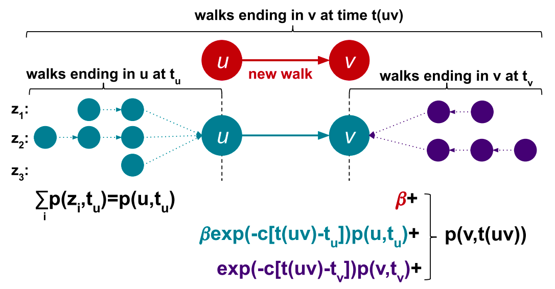
The weight of the node and probability for walk sampling are like two sides of the same coin. They represent a sum over all temporal walks z ending in node v using edges arriving no later than the latest one of already sampled ones in the temporal walk. When the algorithm decides which edge to take next for temporal walk creation, it uses these computed weights (probabilities). Every time a new edge appears in the graph, these probabilities are updated just for two nodes, source and target of the new edge. In Image 4 you can take a look at how probability is updated. For node u we need to check if there were already some walks sampled for it. If there were, make sure to update the weight of node (sum of walks ending in that node) by multiplying with time decayed factor exp(−c · t(uv) − tᵤ).

Here tᵤ represents last time edge pointing to node u appeared in graph, and t(uv) represents time of current edge u⟶v. Afterwards, for node v make sure to sum up the walks from node u, and also walks ending in v multiplied with time decayed factor exp(−c · t(uv) − tᵤ).

This time decayed factor is here to give more weight to nodes with fresher edges.

Word2Vec update

This is the part where we optimize our node embeddings to be as similar as possible. We also make use of the word2vec method mentioned earlier.

After walks sampling, we use these prepared temporal walks to make nodes more similar to those nodes in their temporal neighborhood. What does this mean? So, let's say that our maximum walk length walk_length is set to 4, and the number of walks walk_num is set to 3. These hyperparameters can be found in our implementation of Dynamic Node2Vec on GitHub. Let's imagine we sampled the following temporal walks for node 9 in the graph on Image 3: [1,2,6,9], [1,2,5,9], [5,7,9]

Don't forget that this walk_length is the maximum length. Walk length can also be shorter. Now we need to make our embedding of node 9 most similar to nodes that appeared in that temporal walk. So in math terms, this would mean the following: we seek to optimize the objective function which maximizes the logarithmic probability of observing a network neighborhood Nₛ(u) for node u based on its feature representation (representation in embedded space). Also, we make some assumptions for the problem to be easier to imagine out. This is the formula:

Here Pr(Nₛ(u) | f(u)) is a probability of observing neighborhood nodes of node u with a condition that we are currently in embedded space in place of node u. For example, if the embedded space of node u is vector [0.5, 0.6], and imagine you are at that point, what is the likelihood to observe neighborhood nodes of node u. For each node (that's why there is summation), we want to make the probability as high as possible.

It sounds complicated, but with the following assumptions, it will get easier to comprehend:

1. The first one is that observing a neighborhood node is independent of observing any other neighborhood node given its feature representation. For example, in Image 3, there is a probability for us to observe nodes 6, 7, and 8 if we are on node 9. This is just a relaxation for optimization purposes used often in machine learning which makes it easier for us to compute the above mentioned probability Pr(Nₛ(u) | f(u)). Our probabilities (weights) from the chapter of Probabilities (weights) update are already incorporated in walk sampling. This relaxation is here just for probability calculation.

2. The second one is that observing the source node and neighborhood node in the graph is the same as observing feature representation (embedding of the source node and feature representation of the neighborhood node in feature space. Take a note that in the probability calculation Pr(Nₛ(u)|f(u)) we mentioned feature representation of node f(u) and regular nodes, which sounds like comparing apples and oranges, but with the following relaxation, it should be the same. So for some neighborhood node nᵢ in the neighborhood Nₛ of node u we could have the following:

The exponential term ensures that the sum of probabilities of every neighborhood node of node u is 1. This is also called a softmax function.

This is our optimization problem. Now, we hope that you have an idea of what our goal is. Luckily for us, this is already implemented in a Python module called gensim. Yes, these guys are brilliant in natural language processing and we will make use of it. 🤝

Conclusion

Dynamic node2vec offers a good solution for growing networks. We learned where embeddings can be applied, we mentioned the drawbacks of static graph embedding algorithms and learned about the benefits of dynamic node2vec. All that's left is to try it out yourself.

Our team of engineers is currently tackling the problem of graph analytics algorithms on real-time data. If you want to discuss how to apply online/streaming algorithms on connected data, feel free to join our Discord server and message us.

MAGE shares his wisdom on a Twitter account. Get to know him better by clicking the follow button! 🐦

Last but not least, check out MAGE and don’t hesitate to give a star ⭐ or contribute with new ideas.